Amdahls Law How is system performance altered when some component is - PowerPoint PPT Presentation

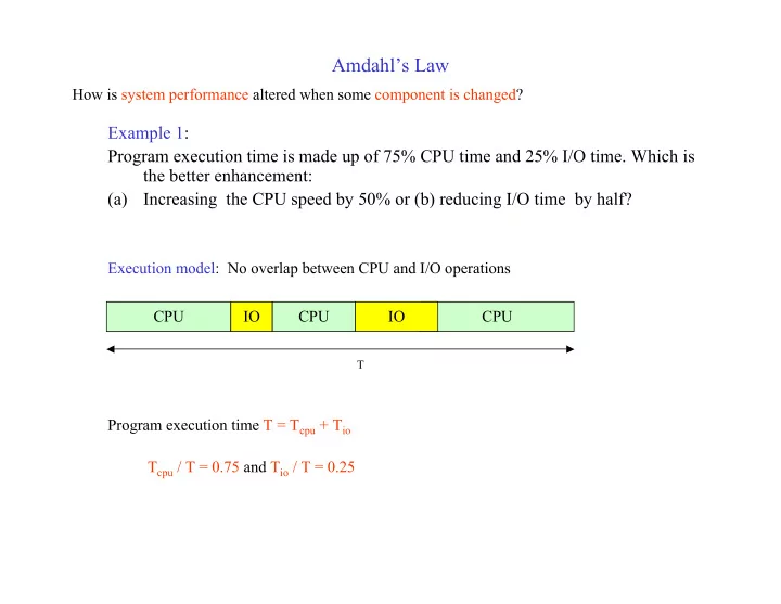
Amdahl’s Law How is system performance altered when some component is changed? Example 1: Program execution time is made up of 75% CPU time and 25% I/O time. Which is the better enhancement: (a) Increasing the CPU speed by 50% or (b) reducing I/O time by half? Execution model: No overlap between CPU and I/O operations CPU IO CPU IO CPU T Program execution time T = T cpu + T io T cpu / T = 0.75 and T io / T = 0.25

Amdahl’s Law (a) Increasing the CPU speed by 50% Program execution time T = T cpu + T io T old = T T cpu / T = 0.75 T io / T = 0.25 T CPU IO CPU IO CPU a b CPU IO CPU IO CPU b 2a/3 Program execution time T new = T cpu / 1.5 + T io T new = T cpu / 1.5 + T io = 0.75 T / 1.5 + 0.25T = 0.75T For a 50% improvement in CPU speed: Execution time decreases by 25% Speedup = T old / T new = T/ 0.75T = 1.33

Amdahl’s Law (b) Halve the IO Time Program execution time T = T cpu + T io T old = T T cpu / T = 0.75 T io / T = 0.25 T CPU IO CPU IO CPU a b CPU IO CPU IO CPU a b/2 Program execution time T new = T cpu + T io / 2 T new = 0.75 T + 0.25T /2 = 0.875T For a 100% improvement in IO speed: Execution time decreases by 12.5% Speedup = T old / T new = T/ 0.875T = 1.14

Amdahl’s Law Limiting Cases CPU speed improved infinitely so T CPU tends to zero • T new = T IO = 0.25T Speedup limited to 4 IO speed improved infinitely so T IO tends to zero • T new = T CPU = 0.75T Speedup limited to 1.33

Amdahl’s Law Example 2: Parallel Programming (Multicore execution) A program made up of 10% serial initialization and finalization code. The remainder is a fully parallelizable loop of N iterations. INITIALIZATION CODE for (j = 0; j < N; j++) { a[j] = b[j] + c[j]; d[j] = d[j] * c; } FINALIZATION CODE T = T INIT + T LOOP + T FINAL = T SERIAL + T LOOP 3

Amdahl’s Law Each iteration can be executed in parallel with the other iterations Assuming p = 4 + a[0] b[0] c[0] for (j = 0; j < 25; j++) { + a[1] b[1] c[1] a[j] = b[j] + c[j]; d[j] = d[j] * c; } + a[23] b[23] c[23] + a[24] b[24] c[24] + a[25] b[25] c[25] + a[26] b[26] c[26] for (j = 25; j < 50; j++) { a[j] = b[j] + c[j]; d[j] = d[j] * c; + } a[48] b[48] c[48] + a[49] b[49] c[49] + a[50] b[50] c[50] + a[51] b[51] c[51] for (j = 50; j < 75; j++) { a[j] = b[j] + c[j]; d[j] = d[j] * c; } + a[73] b[73] c[73] + a[74] b[74] c[74] + a[75] b[75] c[75] for (j = 75; j < 100; j++) { + a[76] b[76] c[76] a[j] = b[j] + c[j]; d[j] = d[j] * c; 3 + a[98] b[98] c[98] } a[99] b[99] c[99] +

Amdahl’s Law Example 2: Parallel Programming (Multicore execution) INITIALIZATION CODE Start Multiple threads FORK for (j = 0; j < 25; j++) { for (j = 25; j < 50; j++) { for (j = 50; j < 75; j++) { for (j = 75; j < 100; j++) { a[j] = b[j] + c[j]; a[j] = b[j] + c[j]; a[j] = b[j] + c[j]; a[j] = b[j] + c[j]; d[j] = d[j] * c; d[j] = d[j] * c; d[j] = d[j] * c; d[j] = d[j] * c; } } } } End Multiple threads JOIN FINALIZATION CODE 3

Amdahl’s Law Performance Model Assume – System Calls for FORK/JOIN incur zero overhead – Execution time for parallel loop scales linearly with the number of iterations in the loop • With p processors executing the loop in parallel Each processor executes N/p iterations Parallel time for executing the loop is : T LOOP / p Sequential time: T SEQ = T T = T SERIAL + T LOOP T SERIAL = 0.1 T T LOOP = 0.9T T p = T SERIAL + T LOOP / p Parallel Time with p processors: = 0.1T + 0.9T/p

Amdahl’s Law Performance Model Parallel Time with p processors: T p = T SERIAL + T LOOP / p T p = 0.1T + 0.9T/p p = 2: T p = 0.1T + 0.9T/p = 0.55 T Speedup = T/0.55T = 1.8 p = 4: T p = 0.1T + 0.9T/p = 0.325 T Speedup = T/0.325T = 3.0 p = 8: T p = 0.1T + 0.9T/p = 0.2125 T Speedup = T/0.2125T = 4.7 p = 16: T p = 0.1T + 0.9T/p = 0.15625 T Speedup = T/0.15625T = 6.4 Limiting Case: p so large that T LOOP is negligible (assume 0) T p = 0.1T and Maximum Speedup is 10!! Program with a fraction f of serial (non-parallelizable) code will have a maximum speedup of 1/f

Amdahl’s Law Diminishing Returns Adding more processors leads to successively smaller returns in terms of • speedup Using 16 processors does not results in an anticipated 16-fold speedup • The Non-parallelizable sections of code takes a larger percentage of the • execution time as the loop time is reduced Maximum Speedup is theoretically limited by fraction f of serial code • So even 1% serial code implies speedup of 100 at best! • Q: In the light of this pessimistic assessment: Why is multicore alive and well and even becoming the dominant paradigm?

Amdahl’s Law Why is multicore alive and well and even becoming the dominant paradigm? 1. Throughput Computing: Run large numbers of independent computations (e.g. Web or Database transactions) on different cores 2. Scaling Problem Size: Use parallel processing to solve larger problem sizes in a given amount of time • Different from solving a small problem even faster • In many situations scaling the problem size (N in our example) does not imply a proportionate increase in the serial portion. , Serial fraction f drops as problem size is increased Examples: • Opening a file is a fixed serial overhead independent of problem size • The fraction it represents decreases as the problem size is increased Parallel IO is routinely available today while it used to be a serialized overhead • Sophisticated parallel algorithms / compiler techniques are able to parallelize what used • to be considered intrinsically serial in the past

Amdahl’s Law Summary • How is system performance altered when some component of the design is changed? • Performance Gains (Speedup) by enhancing some design feature – Base design time: T base – Several design components C 1 , C 2 .. C n – Component C k takes fraction f k of the total time – Suppose C k speeded up by factor S; others remain the same – Enhanced design time: T enhanced Base Design Enhanced Design – Time for C k : T base x f k T base x f k /S – Time for rest: T base x(1 - f k ) T base (1 - f k ) – Total Time: T base T base (f k /S + 1- f k ) Speedup = T base / T enhanced = T base / T base (f k / S + 1 - f k ) = 1 / ( (1 - f k ) + f k / S) – As S becomes large Speedup tends to 1/(1-f) asymptotically