Algorithm runtime analysis and computational tractability As soon - PowerPoint PPT Presentation

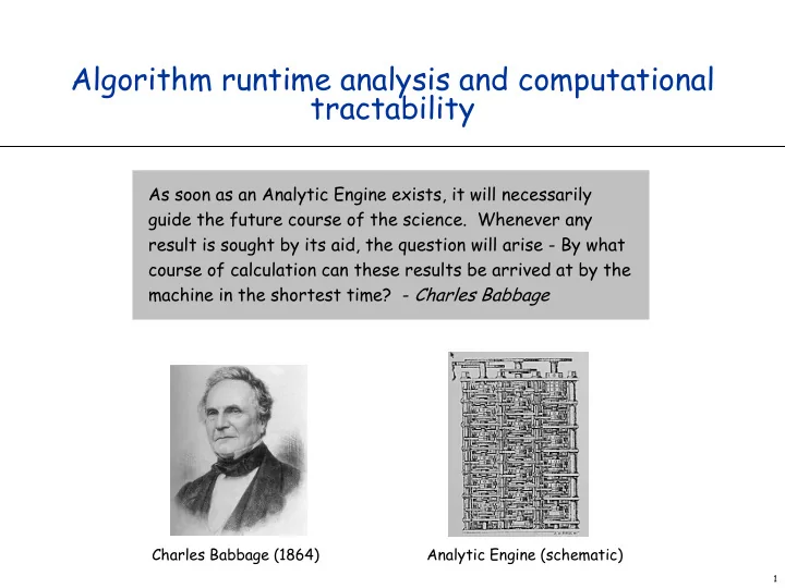
Algorithm runtime analysis and computational tractability As soon as an Analytic Engine exists, it will necessarily guide the future course of the science. Whenever any result is sought by its aid, the question will arise - By what course of calculation can these results be arrived at by the machine in the shortest time? - Charles Babbage Charles Babbage (1864) Analytic Engine (schematic) 1

Time Complexity of an Algorithm How do we measure the complexity (time, space requirements) of an algorithm. The size of the problem: an integer n – # inputs (for sorting problem) – # digits of input (for the primality problem) – sometimes more than one integer o Knapsack problem: –C: capacity of the knapsack, –N: number of objects We want to characterize the running time of an algorithm for increasing problem sizes by a function T(n)

Units of time 1 microsecond ? 1 machine instruction? # of code fragments that take constant time?

Units of time 1 microsecond ? no, too specific and machine dependent 1 machine instruction? no, still too specific and machine dependent # of code fragments that take constant time? yes # what kind of instructions take constant time? arithmetic op, memory access, finite combination of these

unit of space bit? int?

unit of space bit? very detailed but sometimes necessary int? nicer, but dangerous: we can code a whole program or array (or disk) in one arbitrary sized int, so we have to be careful with space analysis (take value ranges into account when needed). Better to think in terms of machine words i.e. fixed size, e.g. 64, collections of bits

Worst-Case Analysis Worst case running time. A bound on largest possible running time of algorithm on inputs of size n. ■ Generally captures efficiency in practice, but can be an overestimate. Same for worst case space complexity 7

Average case Average case running time. A bound on the average running time of algorithm on random inputs as a function of input size n. In other words: the expected number of steps an algorithm takes. ∑ P . C i i i ∈ I n P i : probability input i occurs C i : complexity given input i I n : all possible inputs of size n ■ Hard to model real instances by random distributions. ■ Algorithm tuned for a certain distribution may perform poorly on other inputs. ■ Often hard to compute. 8

Why It Matters 9

A definition of tractability: Polynomial-Time Brute force. For many problems, there is a natural brute force search algorithm that checks every possible solution. ■ Typically takes exponential time for inputs of size n. ■ Unacceptable in practice. – Permutations, TSP An algorithm is said to be polynomial if there exist constants c > 0 and d > 0 such that on every input of size n, its running time is bounded by c n d steps. ■ What about an n log n algorithm? 10

Worst-Case Polynomial-Time On the one hand: ■ Possible objection: Although 6.02 ´ 10 23 ´ n 20 is technically poly-time, it would be useless in practice, (e.g. n=10) ■ In practice, the poly-time algorithms that people develop typically have low constants and low exponents . ■ Breaking through the exponential barrier of brute force typically exposes some crucial structure of the problem. On the other: ■ Some exponential-time (or worse) algorithms are widely used because the worst-case (exponential) instances seem to be rare. simplex method solving linear programming problems • 11

Characterizing algorithm running times Suppose that algorithm A has a running time bounded by T(n) = 1.62 n 2 + 3.5 n + 8 v There is more detail than is useful We want to quantify running time in a way that will v allow us to identify broad classes of algorithms v I.e., we only care about Orders of Magnitude and only consider the leading factor in this case : T(n) = O(n 2 ) v

Asymptotic Growth Rates

Upper bounds Recap from cs220: T(n) is O(f(n)) if there exist constants c > 0 and n 0 ³ 0 such that for all n ³ n 0 : T(n) £ c · f(n) Example: T(n) = 32n 2 + 16n + 32. ■ T(n) is O(n 2 ) ■ BUT ALSO: T(n) is O(n 3 ), T(n) is O(2 n ). There are many possible upper bounds for one function! We always look for the best (lowest) upper bound. 14

Expressing Lower Bounds Big O doesn’t always express what we want: Any comparison-based sorting algorithm requires at least c(n log n) comparisons, for some constant c. ■ Use W for lower bounds. T(n) is W (f(n)) if there exist constants c > 0 and n 0 ³ 0 such that for all n ³ n 0 :T(n) ³ c · f(n) Example: T(n) = 32n 2 + 16n + 32. ■ T(n) is W (n 2 ) 15

Tight Bounds T(n) is Q (f(n)) if T(n) is both O(f(n)) and W (f(n)). Example: T(n) = 32n 2 + 17n + 32. ■ T(n) is Q (n 2 ). If we show that the running time of an algorithm is Q (f(n)), we have closed the problem and found a bound for the problem and its algorithm solving it. 16

G(n) F(n) is O(G(n)) F(n) is W (H(n)) F(n) if G(n) = c.H(n) then F(n) is Q (G(n)) H(n) These measures were introduced in CS220 17

Excursion: heaps and priority queues priority Queue : data structure that maintains a set S of elements. Each element v in S has a key key(v) that denotes the priority of v. Priority Queue provides support for inserting , deleting elements, selection / extraction of smallest (Min prioQ) or largest (Max prioQ) key element, changing key value.

Applications E.g. used in managing real time events where we want to get the earliest next event and events are added and deleted on the fly. Also used in Sorting: ■ build a prioQ ■ Iteratively extract the smallest element PrioQs can be implemented using heaps

Heaps Heap: array representation of a Complete Binary tree every level is completely filled except the ■ 16 bottom level: filled from left to right ■ Can compute the index of parent and 10 14 children: WHY? 8 7 9 – parent(i) = floor((i-1)/2) 3 leftChild(i)= 2i+1 2 1 4 rightChild(i)=2(i+1) 16 14 10 8 7 9 3 2 4 1 0 1 2 3 4 5 6 7 8 9 Max Heap property: for all nodes i>0: A[parent(i)] >= A[i] Max heaps have the max at the root Min heaps have the min at the root

Heapify(A,i,n) To create a heap at index i, assuming left(i) and right(i) are heaps, bubble A[i] down : swap with max child until heap property holds heapify(A,i,n): # precondition # n is the size of the heap # tree left(i) and tree right(i) are heaps ……. # postcondition: tree A[i] is a heap

Swapping Down Swapping down enforces (max) heap property at the swap location: new x y y new x new<x and y<x: x>y and x>new swap(x,new) Are we done now? NO! When we have swapped we need to carry on checking whether new is in heap position. We stop when that is the case. 22

Heap Extract Heap extract: Delete (and return) the root Step 1: replace root with last array element to keep completeness Step 2: reinstate the heap property Which element does not necessarily have the heap property? How can it be fixed? Complexity? heapify the root O(log n) Swap down: swap with maximum (maxheap), minimum (minheap) child as necessary, until in place. Sometimes called bubble down Correctness based on the fact that we started with a heap, so the children of the root are heaps 23

Heap Insert Step 1 : put a new value into first open position (maintaining completeness), i.e. at the end of the array, but now we potentially violated the heap property, so: Step 2 : bubble up ■ Re-enforcing the heap property ■ Swap with parent, if new value > parent, until in the right place. ■ The heap property holds for the tree below the new value, when swapping up. WHY? We only compared the new element to the parent, not to the sibling! 24

Swapping up Swapping up enforces heap property for the sub tree below the new, inserted value: x new y new y x if (new > x) swap(x,new) x>y, therefore new > y 25

Building a heap heapify performs at most lg n swaps why? what is n? buildheap: builds a heap out of an array: ■ the leaves are all heaps WHY? ■ heapify backwards starting at last internal node WHY backwards? WHY last internal node? which node is that?

LET’S DO THE BUILDHEAP! 4 4 7 8 7 8 [4, 8, 7, 2, 14, 1] 2 14 1 2 14 1 4 14 14 7 14 7 4 7 8 2 8 1 2 8 1 2 4 1

NOW LET’S ADD 18 Build heap [4, 8, 7, 2, 14, 1] add 18 bubble up (2*) 18 14 14 14 8 7 7 8 8 7 2 4 1 18 2 4 2 1 4 1

NOW LET’S EXTRACT MAX Delete max (18) move 7 to root bubble down (1*) 7 18 14 14 8 14 14 8 8 7 8 7 2 4 1 7 2 4 1 2 4 1 2 4 1

Complexity buildheap Initial thought: O(n lgn), but half of the heaps are height 0 quarter are height 1 only one is height log n It turns out that O(n lgn) is not tight!

complexity buildheap max #swaps ? height 0 1 2 3

complexity buildheap max #swaps, see a pattern? height (What kind of growth function do you expect ?) 0 0 1 1 2 2*1+2 = 4 3 2*4+3 = 11

complexity buildheap height max #swaps 0 0 = 2 1 -2 1 1 = 2 2 -3 2 2*1+2 = 4 = 2 3 -4 3 2*4+3 = 11 = 2 4 -5