
SLIDE 1
Algorithmic Game Theory CoReLab (NTUA) Lecture 3: Tractability of - - PowerPoint PPT Presentation
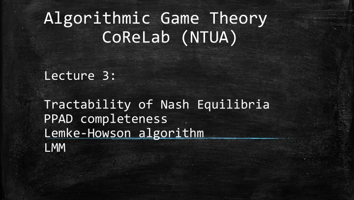
Algorithmic Game Theory CoReLab (NTUA) Lecture 3: Tractability of Nash Equilibria PPAD completeness Lemke-Howson algorithm LMM So far NE in 2-player zero sum LP Duality Nashs Theorem (1950) Every (finite) game has a Nash
Sperner Brouwer Nash
The problem resisted polynomial algorithms for a long time which altered the research direction towards hardness results. The first idea would be to prove Nash an FNP-complete problem. But accepting an FSAT Nash reduction directly implies NP=coNP. (!)
What prevented our previous attempt was the fact that Nash problem always has solution. So the next idea would be to prove it complete for this class. But no complete problem is known for TFNP.
In order to overcome the obstacles we face we need to work as follows:
complete for the class.
No matter how the internal nodes are colored there exists a tri-chromatic triangle. In fact there will be an
no blue no yellow no red
We have to work with a graph of exponential size!
Input: 2 n-bit x numbers y yes/no
Circuit
2𝑜 2𝑜
artificial vertex on the bottom left
directed walk crossing red-yellow doors having red on
Graph Representation
▪ Every vertex has in and out degree at most 1 ▪ Each vertex with degree 1 is an acceptable solution (except the artificial one) ▪ By the parity argument there is always an even number of solutions ▪ Notice that if we insist in finding the pair of our green node the problem is beyond FNP! ...
END OF THE LINE
node id node id node id node id Given F and C : If 0n is an unbalanced node, find another unbalanced node. Otherwise say “yes”.
father child
PPAD = { Search problems in FNP reducible to END OF THE LINE}
𝐺 𝑤2 = 𝑤1 ˄ 𝐷 𝑤1 = 𝑤2
FNP NP=coNP
TFNP Semantic
PPAD Sperner Brouwer Nash
[Daskalakis,Goldberg,Papadimitriou 2006]
...
0n
Generic PPAD
[Pap ’94] [DGP ’05]
Embed PPAD graph in [0,1]3
[DGP ’05]
3D-SPERNER
:=
xa >
Arithmetic Circuit Sat Polymatrix game [DGP ’05] [DGP ’05] [DGP ’05]
, , , , , }
:= +
×a >
Comparison gate: 𝑧 == 1, 𝑗𝑔 𝑦1 > 𝑦2 0, 𝑗𝑔 𝑦1 < 𝑦2 ∗, 𝑗𝑔 𝑦1 = 𝑦2 ▪ Example :
1/3
𝑦1 > := 𝑦2 𝑦3
Unique solution: 𝑦1 = 𝑦2 = 𝑦3 = 1 3
constraints by 𝜗 ≥ 0: Assignment : 𝑧 == 𝑦1 ± 𝜗 Set to const : 𝑧 == max{0, min 𝑏, 1 } ± 𝜗 Addition : 𝑧 == min 1, 𝑦1 + 𝑦2 ± 𝜗 Multiply const: 𝑧 == max{0, min 𝑏𝑦, 1 } ± 𝜗 Subtraction : 𝑧 == max 0, 𝑦1 − 𝑦2 ± 𝜗 Comparison gate: 𝑧 == 1, 𝑗𝑔 𝑦1 > 𝑦2 − 𝜗 0, 𝑗𝑔 𝑦1 < 𝑦2 + 𝜗 ∗, 𝑗𝑔 𝑦1 = 𝑦2 ± 𝜗 Both versions of the problem are PPAD-complete!
the strategies of the players pointing to her.
𝑣𝑤 𝑦1, 𝑦2, … , 𝑦𝑜 =
(𝑥,𝑤)∈𝐹
𝑣𝑥,𝑤(𝑦𝑥, 𝑦𝑤)
Games, we will present polymatrix gadgets which simulate the arithmetic functions of the circuit.
feasible solution of Arithmetic Circuit Sat.
𝑦 𝑨 𝑥 𝑧 Variable nodes
Gate node
𝑣 𝑥: 0 = Pr 𝑦: 1 + Pr[𝑧: 1] 𝑣 𝑥: 1 = Pr[z: 1] 𝑣 𝑨: 0 = 0.5 𝑣 𝑨: 1 = 1 − Pr[𝑥: 1] In any Nash equilibrium of a game containing this Gadget Pr z: 1 = min{1, Pr x: 1 + Pr y: 1 }
𝑣 𝑥: 0 = Pr 𝑦: 1 + Pr[𝑧: 1] 𝑣 𝑥: 1 = Pr[z: 1] 𝑣 𝑨: 0 = 0.5 𝑣 𝑨: 1 = 1 − Pr[𝑥: 1]
Pr[𝑨: 1] = min{1, Pr[𝑦: 1] + Pr[𝑧: 1]}
𝑦 z 𝑧 Variable nodes 𝑣 𝑨: 0 = Pr 𝑧: 1 𝑣 𝑨: 1 = Pr[x: 1]
Pr 𝑦: 1 > Pr[𝑧: 1] Pr 𝑨: 1 = 1 Pr 𝑦: 1 < Pr[𝑧: 1] Pr[𝑨: 1] = 0 Pr[𝑦:1] = Pr 𝑧: 1 anything is possible
𝑦 𝑨 𝑥 𝑧 Variable nodes
Gate node
Every gadget can be turned into a bipartite graph with variable node-players sharing the same side and gate node-players on the
In order to analyze the Lawyer Game we will first define and analyze two games, that combined will give us the appropriate game. Our goal : If (𝑦, 𝑧) is a Nash Equilibrium for the Lawyer Game, then the marginal distributions that 𝑦 assigns to the strategies of the yellow nodes and the marginal distributions that 𝑧 assigns to the red nodes comprise a Nash Equilibrium in the Polymatrix Game.
▪ The Representation Game: The set of strategies for the yellow lawyer is the union of the strategies of every yellow node. The same goes for the red lawyer. The payoff for the lawyers is the payoff that their clients would had gotten had they played the same strategies themselves. ▪ The High Stakes Chase The sets of strategies remain the same. Image an arbitrary labelling {1, . . , 𝑜} for the yellow clients and a respective labelling 1, … , 𝑜 for the red clients. Whenever both lawyers get to pick the same label, the red lawyer pays M to the yellow. Otherwise they both get 0.
M,-M 𝟏, 𝟏 𝟏, 𝟏 𝟏, 𝟏 𝟏, 𝟏 M,-M 𝟏, 𝟏 𝟏, 𝟏 𝟏, 𝟏 𝟏, 𝟏 M,-M 𝟏, 𝟏 𝟏, 𝟏 𝟏, 𝟏 𝟏, 𝟏 M,-M
Given this observation we could claim Proposition 1: Taking M arbitrarily big would essentially lead the lawyers to play with probability (approximately) 1/𝑜 each of their clients in the Combined Game! It is easy to see that the High Stake Chase is a zero-sum game where in every NE the lawyers play uniformly
(We no longer have to worry about our marginal distributions being ill-defined)
Strategies of red node i Strategies
node j
The Representation Game On the other hand if both lawyers play uniformly over their clients, the way that the probability is split among each client’s strategies will not affect the High Stakes Game. The split will be solely determined by the Representation Game and this directly implies that our marginal distributions are indeed a NE for the Polymatrix Game. Notice that we are being a little bit inaccurate as Proposition 1 holds up to an error 𝜗, but the sketch remains the same and the error can be accommodated by the Approximate Arithmetic Circuit Sat!
TFNP
node id { node id1 , node id2}
n-bit input 2n-bit
𝑤1 ∈ 𝑂 𝑣2 & 𝑣2 ∈ 𝑂(𝑣1)
Given N: If 0n has odd degree, find another node with odd degree. Otherwise say “yes”.
PPA = { Search problems in FNP reducible to ODD DEGREE NODE}
Graph Representation
{0,1}n ... 0n
‘Every DAG must have a sink.’
node id {node id1, …, node idk}
node id
‘Every DAG must have a sink.’
n-bit input kn-bit
𝑤2 = 𝑂 𝑤1 & 𝑊 𝑤2 > 𝑊(𝑤1)
FIND SINK Given N, V: Find x s.t. 𝑊(𝑦) ≥ 𝑊(𝑧), for all y N(x). PLS = { Search problems in FNP reducible to FIND SINK}
Graph Representation
{0,1}n
Exponentially large directed acyclic graph
“If a function maps n elements to n-1 elements, then there is a collision.”
node id node id COLLISION Given F: Find x s.t. F( x )= 0n; or find x ≠ y s.t. F(x)=F(y). PPP = { Search problems in FNP reducible to COLLISION }
A bimatix game represented by two matrices 𝐵, 𝐶 is called Symmetric if 𝐶 = 𝐵𝑈 (i.e., the two players have the same set of strategies and their utilities remain the same if their roles are reversed). A strategy profile 𝑦 is a Symmetric Nash Equilibrium if both players playing 𝑦 results in a Nash Equilibrium. Looking at Symmetric Games is no loss of generality!
Fix any bimatrix game represented by the matrices 𝐵, 𝐶 (w.l.o.g. with positive entries). Now consider the Symmetric Game defined by the matrices below:
𝟏 𝑩 𝑪𝑼 𝟏
𝟏 𝑪 𝑩𝐔 𝟏
𝑦 𝑦 𝑧 𝑧 Let 𝑦, 𝑧 be a Symmetric NE. In order 𝑦, 𝑧 to be a best response to itself, 𝑦 must be a best response to 𝑧 and vice versa.
1. A strategy 𝑗 is represented at vertex 𝑨 if 𝑨𝑗 = 0 or 𝐵𝑗𝑨 = 1 or both. 2. Define set 𝑊 with all the vertices of 𝑄 that represent every strategy except possibly strategy 𝑜 3. Any vertex (other than 𝟏) at which all strategies are represented is a NE. 4. In order to find such a vertex we shall develop a (simplex-like) pivoting method beginning at vertex 𝟏 and ending at a SNE.
This vertex represents every strategy It follows that here we get a SNE
𝑨𝑗 = 0 𝐵𝑗𝑨 = 1 𝑨1 = 0 𝑨2 = 0 𝑨3 = 0 …. 𝑨𝑜 = 0
𝑤0
𝑨4 = 0 Choose next inequality to relax
𝑨1 = 0 𝑨2 = 0 𝑨3 = 0 𝐵3𝑨 = 1 𝑨4 = 0 …. Choose next inequality to relax
𝑤𝑙
𝑨2 = 0 𝐵3𝑨 = 1 𝑨4 = 0 …. 𝐵1𝑨 = 1 𝐵𝑜𝑨 = 1 Symmetric Nash Equilibrium!
▪ NE in 2-player zero sum ↔ LP Duality ▪ NE in general 2-player games PPAD complete
( Lemke-Howson exponential running time algorithm )
In order to sidestep the probable intractability of NE we are going to relax
Main result For any NE 𝑦∗, 𝑧∗ and for any 𝜁 > 0, there exists, for every 𝑙 ≥
12 ln 𝑜 𝜁2 a
pair of 𝑙 −uniform strategies 𝑦′, 𝑧,′ such that:
in the NE)
Proof Sketch via Probabilistic Method ▪ Given 𝑦∗, 𝑧∗, 𝜁 > 0 fix 𝑙 ≥
12 ln 𝑜 𝜁2
▪ Form multiset 𝑌 sampling 𝑙 times independently, from the pure strategies of the row player according to the distribution 𝑦∗. Respectively, form 𝑍 from the pure strategies of the column player. ▪ Let 𝑦′ be the 𝑙 −uniform strategy related with multiset 𝑌 and 𝑧′ the 𝑙 −uniform strategy related with multiset 𝑍.
Proof Sketch via Probabilistic Method ▪ Finally consider the following events:
<
𝜁 2}
<
𝜁 2}
𝑜
𝑜
Proof Sketch via Probabilistic Method In order to bound the probability of 𝜒1
𝑑 we define the following :
𝜒1𝑏 = { 𝑦′, 𝐵𝑧∗ − 𝑦∗, 𝐵𝑧∗ } <
𝜁 4
𝜁 4
The expression (𝑦′, 𝐵𝑧∗) is a sum of 𝑙 independent random variables each of expected value (𝑦∗, 𝐵𝑧∗). Each such random variable takes value between 0 and 1. As a result we can apply Chernoff bounds: Pr[𝜒1𝑏
𝑑 ] ≤ 2𝑓−𝑙𝜁2
8
and similarly Pr[𝜒1𝑐
𝑑 ] ≤ 2𝑓−𝑙𝜁2
8
𝑑 ≤ Pr 𝜒1𝑏 𝑑 ∪ 𝜒1𝑐 𝑑
8
Proof Sketch via Probabilistic Method Using the same toolbox we get the following bounds: Pr 𝜒1
𝑑 ≤ 4𝑓−𝑙𝜁2 8
Pr 𝜒2
𝑑 ≤ 4𝑓−𝑙𝜁2 8
Pr 𝜌1,𝑗
𝑑
≤ 4𝑓−𝑙𝜁2
8 +2𝑓−𝑙𝜁2 2
𝑑
8 +2𝑓−𝑙𝜁2 2
Pr 𝐻𝑃𝑃𝐸𝑑 ≤ Pr 𝜒1
𝑑 + Pr 𝜒2 𝑑 + 𝑗=1
Pr 𝜌1,𝑗
𝑑
+
𝑘=1
Pr 𝜌1,𝑘
𝑑
≤ 8𝑓−𝑙𝜁2
8 + 2𝑜
𝑓−𝑙𝜁2
2 + 4𝑓−𝑙𝜁2 8
< 1
n n
In Anonymous Games a large population of players shares the same strategy set and, while players may have different payoff functions, the payoff of each depends on her
(not the identity of these players). Canonical example: 500 citizens have to decide either to go to the cinema or to the theatre and they
(PTAS) A PTAS is an algorithm which takes an instance of an optimization problem and a parameter 𝜁 > 0 and, in polynomial time, produces a solution that is within a factor 1 + 𝜁 of being optimal. Notice that an algorithm running in time 𝑃 𝑜𝜁−1 or even 𝑃(𝑜exp(𝜁−1)) counts as a PTAS.
(Daskalakis, Papadimitriou ’14) There is a PTAS for the mixed Nash equilibrium problem for normalized anonymous games with a constant number of strategies. More precisely, there exists some function such that, for all 𝜁 > 0, an 𝜁 -Nash equilibrium of a normalized anonymous game of m players and n strategies can be computed in time 𝑛(𝑜,𝜁−1).
algorithms