SLIDE 31 Game Theory
Auctions Levent Ko¸ ckesen
Ko¸ c University
Levent Ko¸ ckesen (Ko¸ c University) Auctions 1 / 27
Outline
1
Auctions: Examples
2
Auction Formats
3
Auctions as a Bayesian Game
4
Second Price Auctions
5
First Price Auctions
6
Common Value Auctions
7
Auction Design
Levent Ko¸ ckesen (Ko¸ c University) Auctions 2 / 27
Auctions
Many economic transactions are conducted through auctions treasury bills foreign exchange publicly owned companies mineral rights airwave spectrum rights art work antiques cars houses government contracts Also can be thought of as auctions takeover battles queues wars of attrition lobbying contests
Levent Ko¸ ckesen (Ko¸ c University) Auctions 3 / 27
Auction Formats
1.1 ascending-bid auction
⋆ aka English auction ⋆ price is raised until only one bidder remains, who wins and pays the
final price 1.2 descending-bid auction
⋆ aka Dutch auction ⋆ price is lowered until someone accepts, who wins the object at the
current price
2.1 first price auction
⋆ highest bidder wins; pays her bid
2.2 second price auction
⋆ aka Vickrey auction ⋆ highest bidder wins; pays the second highest bid Levent Ko¸ ckesen (Ko¸ c University) Auctions 4 / 27
Auction Formats
Auctions also differ with respect to the valuation of the bidders
- 1. Private value auctions
◮ each bidder knows only her own value ◮ artwork, antiques, memorabilia
◮ actual value of the object is the same for everyone ◮ bidders have different private information about that value ◮ oil field auctions, company takeovers Levent Ko¸ ckesen (Ko¸ c University) Auctions 5 / 27
Equivalent Formats
English auction has the same equilibrium as Second Price auction This is true only if values are private Stronger equivalence between Dutch and First Price auctions
Open Bid Sealed Bid Dutch Auction First Price English Auction Second Price
Strategically Equivalent Same Equilibrium in Private Values Levent Ko¸ ckesen (Ko¸ c University) Auctions 6 / 27
Independent Private Values
Each bidder knows only her own valuation Valuations are independent across bidders Bidders have beliefs over other bidders’ values Risk neutral bidders
◮ If the winner’s value is v and pays p, her payoff is v − p Levent Ko¸ ckesen (Ko¸ c University) Auctions 7 / 27
Auctions as a Bayesian Game
set of players N = {1, 2, . . . , n} type set Θi = [v, ¯ v] , v ≥ 0 action set, Ai = R+ beliefs
◮ opponents’ valuations are independent draws from a distribution
function F
◮ F is strictly increasing and continuous
payoff function ui (a, v) = vi−P (a)
m
, if aj ≤ ai for all j = i, and |{j : aj = ai}| = m 0, if aj > ai for some j = i
◮ P (a) is the price paid by the winner if the bid profile is a Levent Ko¸ ckesen (Ko¸ c University) Auctions 8 / 27
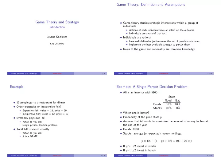
Second Price Auctions
Only one 4.5G license will be sold There are 10 groups I generated 10 random values between 0 and 100 I will now distribute the values: Keep these and don’t show it to anyone until the end of the experiment I will now distribute paper slips where you should enter your name, value, and bid Highest bidder wins, pays the second highest bid I will pay the winner her net payoff: value - price Click here for the EXCEL file
Levent Ko¸ ckesen (Ko¸ c University) Auctions 9 / 27
Second Price Auctions
- I. Bidding your value weakly dominates bidding higher
Suppose your value is $10 but you bid $15. Three cases:
- 1. There is a bid higher than $15 (e.g. $20)
◮ You loose either way: no difference
- 2. 2nd highest bid is lower than $10 (e.g. $5)
◮ You win either way and pay $5: no difference
- 3. 2nd highest bid is between $10 and $15 (e.g. $12)
◮ You loose with $10: zero payoff ◮ You win with $15: loose $2
5 10 value 12 15 bid 20
Levent Ko¸ ckesen (Ko¸ c University) Auctions 10 / 27
Second Price Auctions
- II. Bidding your value weakly dominates bidding lower
Suppose your value is $10 but you bid $5. Three cases:
- 1. There is a bid higher than $10 (e.g. $12)
◮ You loose either way: no difference
- 2. 2nd highest bid is lower than $5 (e.g. $2)
◮ You win either way and pay $2: no difference
- 3. 2nd highest bid is between $5 and $10 (e.g. $8)
◮ You loose with $5: zero payoff ◮ You win with $10: earn $2
2 10 value 8 5 bid 12
Levent Ko¸ ckesen (Ko¸ c University) Auctions 11 / 27
First Price Auctions
Only one 4.5G license will be sold There are 10 groups I generated 10 random values between 0 and 100 I will now distribute the values: Keep these and don’t show it to anyone until the end of the experiment I will now distribute paper slips where you should enter your name, value, and bid Highest bidder wins, pays her bid I will pay the winner her net payoff: value - price Click here for the EXCEL file
Levent Ko¸ ckesen (Ko¸ c University) Auctions 12 / 27
First Price Auctions
Highest bidder wins and pays her bid Would you bid your value? What happens if you bid less than your value?
◮ You get a positive payoff if you win ◮ But your chances of winning are smaller ◮ Optimal bid reflects this tradeoff
Bidding less than your value is known as bid shading
Levent Ko¸ ckesen (Ko¸ c University) Auctions 13 / 27
Bayesian Equilibrium of First Price Auctions
Only 2 bidders You are player 1 and your value is v > 0 You believe the other bidder’s value is uniformly distributed over [0, 1] You believe the other bidder uses strategy β(v2) = av2 Highest possible bid by the other = a: Optimal bid ≤ a Your expected payoff if you bid b (v − b)prob(you win) = (v − b)prob(b > av2) = (v − b)prob(v2 < b/a) = (v − b) b a
Levent Ko¸ ckesen (Ko¸ c University) Auctions 14 / 27
Bayesian Equilibrium of First Price Auctions
Your expected payoff if you bid b (v − b) b a The critical value is found by using FOC: − b a + v − b a = 0 ⇒ b = v 2 This gives a higher payoff than the boundary b = 0 Bidding half the value is a Bayesian equilibrium
Levent Ko¸ ckesen (Ko¸ c University) Auctions 15 / 27
Bayesian Equilibrium of First Price Auctions
n bidders You are player 1 and your value is v > 0 You believe the other bidders’ values are independently and uniformly distributed over [0, 1] You believe the other bidders uses strategy β(vi) = avi Highest bid of the other players = a: Optimal bid b ≤ a Your expected payoff if you bid b (v − b)prob(you win) (v − b)prob(b > av2 and b > av3 . . . and b > avn) This is equal to (v−b)prob(b > av2)prob(b > av3) . . . prob(b > avn) = (v−b)(b/a)n−1
Levent Ko¸ ckesen (Ko¸ c University) Auctions 16 / 27