Algorithm runtime analysis and computational tractability As soon - - PowerPoint PPT Presentation

algorithm runtime analysis and computational tractability
SMART_READER_LITE
LIVE PREVIEW

Algorithm runtime analysis and computational tractability As soon - - PowerPoint PPT Presentation

Algorithm runtime analysis and computational tractability As soon as an Analytic Engine exists, it will necessarily guide the future course of the science. Whenever any result is sought by its aid, the question will arise - By what course of


slide-1
SLIDE 1

Algorithm runtime analysis and computational tractability

1

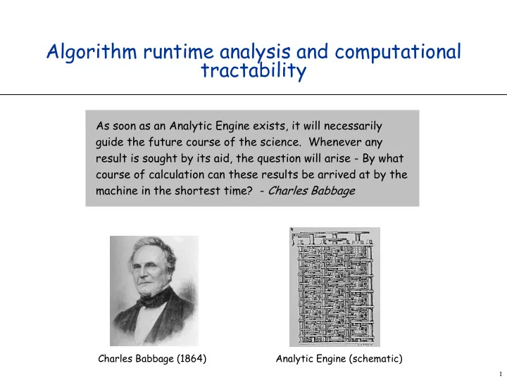
Charles Babbage (1864)

As soon as an Analytic Engine exists, it will necessarily guide the future course of the science. Whenever any result is sought by its aid, the question will arise - By what course of calculation can these results be arrived at by the machine in the shortest time? - Charles Babbage

Analytic Engine (schematic)

slide-2
SLIDE 2

Time Complexity of an Algorithm

How do we measure the complexity (time, space requirements) of an algorithm. The size of the problem: an integer n

– # inputs (for sorting problem) – # digits of input (for the primality problem) – sometimes more than one integer

  • Knapsack problem:

–C: capacity of the knapsack, –N: number of objects We want to characterize the running time of an algorithm for increasing problem sizes by a function T(n)

slide-3
SLIDE 3

Units of time

1 microsecond ? 1 machine instruction? # of code fragments that take constant time?

slide-4
SLIDE 4

Units of time

1 microsecond ? no, too specific and machine dependent 1 machine instruction? no, still too specific and machine dependent # of code fragments that take constant time? yes # what kind of instructions take constant time? arithmetic op, memory access, finite combination of these

slide-5
SLIDE 5

unit of space

bit? int?

slide-6
SLIDE 6

unit of space

bit? very detailed but sometimes necessary int? nicer, but dangerous: we can code a whole program or array (or disk) in one arbitrary sized int, so we have to be careful with space analysis (take value ranges into account when needed). Better to think in terms of machine words

i.e. fixed size, e.g. 64, collections of bits

slide-7
SLIDE 7

7

Worst-Case Analysis

Worst case running time. A bound on largest possible running time of algorithm

  • n inputs of size n.

■ Generally captures efficiency in practice, but can be

an overestimate. Same for worst case space complexity

slide-8
SLIDE 8

Average case

Average case running time. A bound on the average running time of algorithm on random inputs as a function of input size n. In other words: the expected number of steps an algorithm takes.

■ Hard to model real instances by random

distributions.

■ Algorithm tuned for a certain distribution may

perform poorly on other inputs.

■ Often hard to compute. 8

P

i i∈I n

.Ci P

i : probability input i occurs

Ci :complexity given input i In : all possible inputs of size n

slide-9
SLIDE 9

9

Why It Matters

slide-10
SLIDE 10

10

A definition of tractability: Polynomial-Time

Brute force. For many problems, there is a natural brute force search algorithm that checks every possible solution.

■ Typically takes 2n time or worse for inputs of size n. ■ Unacceptable in practice.

– Permutations, TSP

■ What about an n log n algorithm?

An algorithm is said to be polynomial if there exist constants c > 0 and d > 0 such that on every input of size n, its running time is bounded by c nd steps.

slide-11
SLIDE 11

11

Worst-Case Polynomial-Time

On the one hand:

■ Possible objection: Although 6.02 ´ 1023 ´ n20 is technically

poly-time, it would be useless in practice, (e.g. n=10)

■ In practice, the poly-time algorithms that people develop

typically have low constants and low exponents.

■ Breaking through the exponential barrier of brute force

typically exposes some crucial structure of the problem. On the other:

■ Some exponential-time (or worse) algorithms are widely used

because the worst-case (exponential) instances seem to be rare.

  • simplex method solving linear programming problems
slide-12
SLIDE 12

Characterizing algorithm running times

Suppose that algorithm A has a running time bounded by T(n) = 1.62 n2 + 3.5 n + 8

v There is more detail than is useful

v

We want to quantify running time in a way that will allow us to identify broad classes of algorithms

v I.e., we only care about Orders of Magnitude

v

in this case : T(n) = O(n2)

slide-13
SLIDE 13

Asymptotic Growth Rates

slide-14
SLIDE 14

14

Upper bounds

Recap from cs220: T(n) is O(f(n)) if there exist constants c > 0 and n0 ³ 0 such that for all n ³ n0 : T(n) £ c · f(n) Example: T(n) = 32n2 + 16n + 32.

■ T(n) is O(n2) ■ BUT ALSO: T(n) is O(n3), T(n) is O(2n).

There are many possible upper bounds for one function! We always look for the best (lowest) upper bound, but it is not always easy to establish.

slide-15
SLIDE 15

15

Expressing Lower Bounds

Big O doesn’t always express what we want: Any comparison-based sorting algorithm requires at least c(n log n) comparisons, for some constant c.

■ Use W for lower bounds.

T(n) is W(f(n)) if there exist constants c > 0 and n0 ³ 0 such that for all n ³ n0 :T(n) ³ c · f(n)

Example: T(n) = 32n2 + 16n + 32.

■ T(n) is W(n2), W(n).

slide-16
SLIDE 16

16

Tight Bounds

T(n) is Q(f(n)) if T(n) is both O(f(n)) and W(f(n)). Example: T(n) = 32n2 + 17n + 32.

■ T(n) is Q(n2).

If we show that the running time of an algorithm is Q(f(n)), we have closed the problem and found a bound for the problem and its algorithm solving it.

slide-17
SLIDE 17

17

G(n) F(n) H(n)

F(n) is O(G(n)) F(n) is W(H(n)) if G(n) = c.H(n) then F(n) is Q(G(n)) These measures were introduced in CS220

slide-18
SLIDE 18

Recap: rules of the game

■ We are giving you extra time and trials for quiz 1

– Because we want you to be ready for the material in this class

■ You need to know, and be comfortable with, the Pre-requisiate

material

■ You are responsible for all the material in the class

– Readings from the text – Slides – Exercises – Tutorial

18

slide-19
SLIDE 19

Excursion: heap sort and priority queues

priority Queue: data structure that maintains a set S

  • f elements.

Each element v in S has a key key(v) that denotes the priority of v. Priority Queue provides support for adding, deleting elements, selection / extraction of smallest (Min prioQ) or largest (Max prioQ) key element, changing key value.

slide-20
SLIDE 20

Applications E.g. used in managing real time events where we want to get the earliest next event and events are added / deleted on the fly. Sorting

■ build a prioQ ■ Iteratively extract the smallest element

PrioQs can be implemented using heaps

slide-21
SLIDE 21

Heaps

Heap: array representation of a complete binary tree

every level is completely filled except the bottom level: filled from left to right

■ Can compute the index of parent and

children: WHY?

– parent(i) = floor((i-1)/2)

leftChild(i)= 2i+1 rightChild(i)=2(i+1) Max Heap property: for all nodes i>0: A[parent(i)] >= A[i] Max heaps have the max at the root Min heaps have the min at the root

16 10 9 3 1 4 2 7 8 14 16 14 10 8 7 9 3 2 4 1 0 1 2 3 4 5 6 7 8 9

slide-22
SLIDE 22

Heapify(A,i,n)

To create a heap at index i, assuming left(i) and right(i) are heaps, bubble A[i] down: swap with max child until heap property holds

heapify(A,i,n): # precondition # n is the size of the heap # tree left(i) and tree right(i) are heaps ……. # postcondition: tree A[i] is a heap

slide-23
SLIDE 23

Swapping Down

23

Swapping down enforces (max) heap property at the swap location: new<x and y<x: x>y and x>new swap(x,new) Are we done now? x new y new x y NO! When we have swapped we need to carry

  • n checking whether new is in heap position. We

stop when that is the case.

slide-24
SLIDE 24

Heap Extract

Heap extract: Delete (and return) root Step 1: replace root with last array element to keep completeness Step 2: reinstate the heap property Which element does not necessarily have the heap property? How can it be fixed? Complexity? heapify the root O(log n) Swap down: swap with maximum (maxheap), minimum (minheap) child as necessary, until in place.

Sometimes called bubble down

Correctness based on the fact that we started with a heap, so the children of the root are heaps

24

slide-25
SLIDE 25

Heap Insert

Step 1: put a new value into first open position (maintaining completeness), i.e. at the end of the array, but now we potentially violated the heap property, so: Step 2: bubble up

■ Re-enforcing the heap property ■ Swap with parent, if new value > parent, until in the

right place.

■ The heap property holds for the tree below the new

value, when swapping up. WHY? We only compared the new element to the parent, not to the sibling!

25

slide-26
SLIDE 26

Swapping up

26

Swapping up enforces heap property for the sub tree below the new, inserted value: new x y x new y

if (new > x) swap(x,new) x>y, therefore new > y

slide-27
SLIDE 27

Building a heap

heapify performs at most lg n swaps why? what is n? buildheap: builds a heap out of an array:

■ the leaves are all heaps WHY? ■ heapify backwards starting at last internal node

WHY backwards? WHY last internal node? which node is that?

slide-28
SLIDE 28

1 14 2 7 8 4

LERT’S DO THE BUILDHEAP!

1 14 2 7 8 4 1 8 2 7 14 4 1 8 2 7 4 14 1 4 2 7 8 14 [4, 8, 7, 2, 14, 1]

slide-29
SLIDE 29

Complexity buildheap

Suggestions? ...

slide-30
SLIDE 30

Complexity buildheap

Initial thought: O(n lgn), but half of the heaps are height 0 quarter are height 1

  • nly one is height log n

It turns out that O(n lgn) is not tight!

slide-31
SLIDE 31

complexity buildheap

height 1 2 3 max #swaps ?

slide-32
SLIDE 32

complexity buildheap

height 1 2 3 max #swaps, see a pattern? (What kind of growth function do you expect ?) 1 2*1+2 = 4 2*4+3 = 11

slide-33
SLIDE 33

complexity buildheap

height 1 2 3 max #swaps 0 = 21-2 1 = 22-3 2*1+2 = 4 = 23-4 2*4+3 = 11 = 24-5

slide-34
SLIDE 34

complexity buildheap

height 1 2 3 max #swaps 0 = 21-2 1 = 22-3 2*1+2 = 4 = 23-4 2*4+3 = 11 = 24-5

Conjecture: height = h max #swaps = 2h+1-(h+2) Proof: induction base? step: height = (h+1) max #swaps: 2*(2h+1-(h+2))+(h+1) = 2h+2-2h-4+h+1 = 2h+2-(h+3) = 2(h+1)+1-((h+1)+2) n nodes àQ(n) swaps

slide-35
SLIDE 35

See it the Master theorem way T(n) = 2*T(n/2)+ lg n Master theorem

35

Θ(nlg2 2) = Θ(n)

slide-36
SLIDE 36

Heapsort, complexity

heapsort(A): buildheap(A) # O( n ) for i = n-1 downto 1 : # O( ( n ) # put max at end array # max is removed from heap n=n-1 # reinstate heap property # * ( lg n) )

  • heapify: Q(lgn)
  • heapExtract: Q(lg n)
  • buildheap: Q(n)
  • heapsort: Q(n lg n)
  • space: in place: Q(n)
slide-37
SLIDE 37

1 4 2 7 8 14 14 1 2 7 4 8 14 8 2 1 4 7 14 8 7 1 2 4 14 8 7 4 1 2

DO THE HEAPSORT, DO IT, DO IT!

14 8 7 4 1 2 14 8 7 4 1 2

slide-38
SLIDE 38

How not to heapExtract, heapInsert

38

# These "snail" implementations are NOT preserving the algorithm # complexity of extractMin: log n and insert: log n and are therefore # INCORRECT! from a complexity point of view (even though they are # functionally correct). Remember one of the goals of our course: # implementing the algorithms maintaining the analyzed complexity # What are their complexities? def snailExtractMin(A): n = len(A) if n == 0: return None min = A[0] A[0]=A[n-1] A.pop() buildHeap(A) # O(n) return min def snailInsert(A,v): A.append(v) buildHeap(A) # O(n)

slide-39
SLIDE 39

Priority Queues

heaps can be used to implement priority queues:

■ each value associated with a key ■ max priority queue S has operations that maintain

the heap property of S

– max(S) returning max element – Extract-max(S) extracting and returning max

element

– increase key(S,x,k) increasing the key value of x – insert(S,x)

  • put x at end of S
  • bubble x up in place
slide-40
SLIDE 40

40

Back to O, Properties

Transitivity.

■ If f = O(g) and g = O(h) then f = O(h). ■ If f = W(g) and g = W(h) then f = W(h). ■ If f = Q(g) and g = Q(h) then f = Q(h).

Additivity.

■ If f = O(h) and g = O(h) then f + g = O(h). ■ If f = W(h) and g = W(h) then f + g = W(h). ■ If f = Q(h) and g = Q(h) then f + g = Q(h).

slide-41
SLIDE 41

41

Asymptotic Bounds for Some Common Functions

  • Polynomials. a0 + a1n + … + adnd is O(nd) if ad > 0.

Polynomial time. Running time is O(nd) for some constant d

  • Logarithms. loga n is O(logb n) for any constants a, b > 0.

for every x > 0, log n is O(nx).

  • Combinations. Merge sort, Heap sort O(nlogn)
  • Exponentials. For every r > 1 and every d > 0, nd is O(rn).

exponential grows faster than any polynomial can avoid specifying the base log grows slower than any polynomial

slide-42
SLIDE 42

Problems have lower bounds A problem has a lower bound Ω(f(n)), which means : Any algorithm solving this problem takes at least Ω(f(n)) steps We can often show that an algorithm has to "touch" all elements of a data structure, or produce a certain sized output. This then gives rise to an easy lower bound. Sometimes we can prove better (higher, stronger) lower bounds (eg Searching and Sorting (cs420) ).

42

slide-43
SLIDE 43

Closed / open problems

Problems have lower bounds, algorithms have upper

  • bounds. A closed problem has a lower bound Ω(f(n))

and at least one algorithm with upper bound O(f(n))

■ Example: sorting is Ω(n logn) and there are O(n logn)

sorting algorithms. To show this, we need to reason about lower bounds

  • f problems (CS420)

An open problem has lower bound < upper bound

q Example: matrix multiplication (multiply two n x n

matrices).

q

Takes Ω(n2) why?

q

Naïve algorithm: O(n3)

q

Coppersmith-Winograd algorithm: O(n2.376)

slide-44
SLIDE 44

A Survey of Common Running Times

slide-45
SLIDE 45

Constant time: O(1)

A single line of code that involves “simple” expressions, e.g.:

² Arithmetical operations (+,-,*,/) for fixed size

inputs

² assignments (x = simple expression) ² conditionals with simple sub-expressions ² function calls (excluding the time spent in the

called function)

45

slide-46
SLIDE 46

Logarithmic time

Example of a problem with O(log(n)) bound: binary search How did we get that bound?

46

slide-47
SLIDE 47

Guessing game

I have a number between 0 and 63 How many (Y/N) questions do you need to find it? What’s the number? What (kind of) questions would you ask?

47

slide-48
SLIDE 48

Guessing game

I have a number between 0 and 63 How many (Y/N) questions do you need to find it? is it >= 32 N is it >= 16 Y is it >= 24 N is it >= 20 N is it >= 18 Y is it >= 19 Y What’s the number? 19 Take N=0 and Y=1, what is 010011 ?

48

slide-49
SLIDE 49

log(n) and algorithms

When in each step of an algorithm we halve the size

  • f the problem then it takes log2n steps to get to the

base case We often use log(n) when we should use floor(log(n)). That's OK since floor(log(n)) is Q(log(n)) Similarly, if we divide a problem into k equal parts the number of steps is logkn. For the purposes of big-O analysis it doesn’t matter since logan is O(logbn)

slide-50
SLIDE 50

Logarithms

definition: bx = a à x = logba, eg 23=8, log28=3

² log(x*y) = log x + log y because bx by = bx+y ² log(x/y) = log x – log y ² log xa = a log x ² log x is a 1-to-1 monotonically (slow) growing function ² logax = logbx / logba ² ylog x = xlog y

b logb a =a logb b=1 log1=0

log x = log y ⇔ x = y

slide-51
SLIDE 51

logax = logbx / logba

51

blogb x = x = aloga x = b(logb a)(loga x) logb x = (logb a)(loga x) loga x = logb x /logb a

therefore logax = O(logbx) for any a and b

slide-52
SLIDE 52

ylog x = xlog y

52

x logb y = y

logy x logb y =

y(logb x / logb y)logb y = y logb x

slide-53
SLIDE 53

Combinations of functions /code fragments

53

AdditiveTheorem: Sequences of code are additive in complexity: int c = 0; for(int i=0; i<n; i++) c++; for(int j=0; j<m; j++) c++;

Complexity? What is counting the complexity?

Suppose that f1(x) is O(g1(x)) and f2(x) is O(g2(x)). Then ( f1 + f2)(x) is O(max(g1(x),g2(x)).

slide-54
SLIDE 54

Combinations of functions /code fragments

54

Multiplicative Theorem: Nested code is multiplicative in complexity

for(int i=0; i<n; i++) for(int j=0; j<m; j++) c++; Complexity?

BUT, be careful with nests where the inner loop depends outer loop:

int b = n; while(b>0){ b/=2; for(int i=0; i<b; i++) c++; }

Suppose that f1(x) is O(g1(x)) and f2(x) is O(g2(x)). Then ( f1 f2)(x) is O(g1(x)g2(x)).

slide-55
SLIDE 55

Recursive Code

Draw the call tree, and assert the number of nodes in the tree and their individual complexity, as a function of n.

55

slide-56
SLIDE 56

Recursive Code

Draw the call tree, and assert the number of nodes in the tree and their individual complexity, as a function of n.

56

public int divCo(int n){ if(n<=1) return 1; else return 1 + divCo(n-1) + divCo(n-1); } How many recursive calls? How much work per call? What is the role of “return 1” and return 1+…” ? So what does this function count? Big O complexity?

slide-57
SLIDE 57

57

Linear Time: O(n)

Linear time. Running time is proportional to the size of the input. Computing the maximum. Compute maximum of n numbers a1, …, an. Also Q(n) ?

max ¬ a1 for i = 2 to n { if (ai > max) max ¬ ai }

slide-58
SLIDE 58

58

Linear Time: O(n)

  • Merge. Combine two sorted lists A = a1,a2,…,an with

B = b1,b2,…,bn into a single sorted list.

  • Claim. Merging two lists of size n takes O(n) time.

i = 1, j = 1 while (both lists are nonempty) { if (ai £ bj) append ai to output list and increment i else append bj to output list and increment j } append remainder of nonempty list to output list

slide-59
SLIDE 59

Linear Time: O(n)

Polynomial evaluation. Given A(x) = anxn + an-1xn-1 +...+ a1x + a0 (an!=0) Evaluate A(x) How not to do it: an*exp(x,n) + an-1*exp(x,n-1) +...+ a1*x + a0 Why not?

slide-60
SLIDE 60

How to do it: Horner's rule

anx n + an−1x n−1 + ...+ a1x1 + a0 = (anx n−1 + an−1x n−2 + ...+ a1)x + a0 = ... = (...(anx + an−1)x + an−2)x...+ a1)x + a0

y=a[n] for (i=n-1;i>=0;i--) y = y *x + a[i]

slide-61
SLIDE 61

Polynomial evaluation using Horner: complexity Lower bound: Ω(n) because we need to access each a[i] at least once Upper bound: O(n) Closed problem! But what if A(x) = xn

slide-62
SLIDE 62

A(x)=xn

Recurrence: x2n=xn *xn x2n+1=x * x2n Complexity? def pwr(x, n) : if (n==0) : return 1 if odd(n) : return x * pwr(x, n-1) else : a = pwr(x, n/2) return a * a

slide-63
SLIDE 63

A glass-dropping experiment

u You are testing a model of glass jars, and want to

know from what height you can drop a jar without it breaking. You can drop the jar from heights of 1,…,n foot heights. Higher means faster means more likely to break.

u You want to minimize the amount of work (number

  • f heights you drop a jar from). Your strategy

would depend on the number of jars you have available.

v If you have a single jar:

v

do linear search (O(n) work).

v If you have an unlimited number of jars:

v

do binary search (O(log n) work)

v Can you design a strategy for the case you

have 2 jars, resulting in a bound that is strictly less than O(n)?

63

http://xkcd.com/510/

slide-64
SLIDE 64

64

O(n log n) Time

Often arises in divide-and-conquer algorithms like mergesort. mergesort(A) : if len(A) <= 1 return A else return merge(mergesort(left half(A)), mergesort(right half(A)))

slide-65
SLIDE 65

65

Merge Sort - Divide

{7,3,2,9,1,6,4,5} {7,3,2,9} {1,6,4,5} {7,3} {2,9} {1,6} {4,5} {7} {3} {2} {9} {1} {6} {4} {5}

slide-66
SLIDE 66

66

Merge Sort - Merge

{1,2,3,4,5,6,7,9} {2,3,7,9} {1,4,5,6} {3,7} {2,9} {1,6} {4,5} {7} {3} {2} {9} {1} {6} {4} {5}

slide-67
SLIDE 67

O(n log n)

mergesort(A) : if len(A) <= 1 return A else return merge(mergesort(left half(A)), mergesort(right half(A)))

{7} {3} {2} {9} {1} {6} {4} {5} {1,2,3,4,5,6,7,9} {2,3,7,9} {1,4,5,6} {3,7} {2,9} {1,6} {4,5}

How many levels? WHY? At level i

■ work done

– split – merge

total work?

Total depth? Total work?

slide-68
SLIDE 68

Quadratic Time: O(n2)

Quadratic time example. Enumerate all pairs of elements. Closest pair of points. Given a list of n points in the plane (x1, y1), …, (xn, yn), find the pair that is closest. O(n2) solution. Try all pairs of points.

  • Remark. W(n2) seems inevitable, but . . . .

min ¬ (x1 - x2)2 + (y1 - y2)2 for i = 1 to n { for j = i+1 to n { d ¬ (xi - xj)2 + (yi - yj)2 if (d < min) min ¬ d } }

slide-69
SLIDE 69

69

Cubic Time: O(n3)

Example 1: Matrix multiplication Tight? Example 2: Set disjoint-ness. Given n sets S1, …, Sn each of which is a subset of 1, 2, …, n, is there some pair of these which are disjoint? O(n3) solution. For each pairs of sets, determine if they are disjoint. what do we need for this to be O(n3) ?

foreach set Si { foreach other set Sj { foreach element p of Si { determine whether p also belongs to Sj } if (no element of Si belongs to Sj) report that Si and Sj are disjoint } }

slide-70
SLIDE 70

Largest interval sum

Given an array A[0],…,A[n – 1], find indices i,j such that the sum A[i] +… +A[j] is maximized. Naïve algorithm : maximum_sum = - infinity for i in range(n - 1) : for j in range(i, n) : current_sum = A[i] +… +A[j] if current_sum >= maximum_sum : maximum_sum = current_sum save the values of i and j big O bound? Can we do better?

70

Example: A = [2, -3, 4, 2, 5, 7, -10, 8, 12]

slide-71
SLIDE 71

71

Polynomial Time: O(nk) Time

Independent set of size k. Given a graph, are there k nodes such that no two are joined by an edge? O(nk) solution. Enumerate all subsets of k nodes.

■ Check whether S is an independent set = O(k2). ■ Number of k element subsets = ■ O(k2 nk / k!) = O(nk).

foreach subset S of k nodes { check whether S in an independent set if (S is an independent set) report S is an independent set } }

n k " # $ % & ' = n (n−1) (n− 2)  (n− k +1) k (k −1) (k − 2)  (2) (1) ≤ nk k!

poly-time for k=17, but not practical k is a constant

slide-72
SLIDE 72

72

Exponential Time

Independent set. Given a graph, what is the maximum size of an independent set? O(n2 2n) solution. Enumerate all subsets. For some problems (e.g. TSP) we need to consider all

  • permutations. The factorial function (n!) grows much faster

than 2n

S* ¬ f foreach subset S of nodes { check whether S in an independent set if (S is largest independent set seen so far) update S* ¬ S } }

slide-73
SLIDE 73

O(exponential)

Questions

  • 1. Is 2n O(3n) ?
  • 2. Is 3n O(2n)
  • 3. Is 2n O(n!) ?
  • 4. Is n! O(2n)

73

slide-74
SLIDE 74

Polynomial, NP, Exponential

Some problems (such as matrix multiply) have a polynomial complexity solution: an O(np) time algorithm solving them. (p constant) Some problems (such as Hanoi) take an exponential time to solve: Θ(pn) (p constant) For some problems we only have an exponential solution, but we don't know if there exists a polynomial solution. Trial and error algorithms are the only ones we have so far to find an exact solution, and if we would always make the right guess, these algorithms would take polynomial time. We call these problems NP (non deterministic polynomial) We will discuss NP later.

slide-75
SLIDE 75

Some NP problems

TSP: Travelling Salesman given cities c1,c2,...,cn and distances between all of these, find a minimal tour connecting all cities. SAT: Satisfiability given a boolean expression E with boolean variables x1,x2,...,xn determine a truth assignment to all xi making E true

slide-76
SLIDE 76

Back tracking

Back tracking searches (walks) a state space, at each choice point it guesses a choice. In a leaf (no further choices) if solution found OK, else go back to last choice point and pick another move. NP is the class of problems for which we can check in polynomial time whether it is correct (certificates, later)

slide-77
SLIDE 77

Coping with intractability

NP problems become intractable quickly TSP for 100 cities? How would you enumerate all possible tours? How many? Coping with intractability:

■ Approximation: Find a nearly optimal tour ■ Randomization: use a probabilistic algorithm using

"coin tosses" (eg prime witnesses)