Administrivia Homework 5 posted Due April 26, 5:00 PM (note the - PowerPoint PPT Presentation

Administrivia • Homework 5 posted • Due April 26, 5:00 PM (note the change in time) • Last day of class (don’t skip class to do the homework) CMPSCI 370: Intro. to Computer Vision • No HH section today Image representation University of Massachusetts, Amherst April 12/14, 2016 • In the remaining five classes Instructor: Subhransu Maji • Image representations (this week) • Convolutional neural networks (next week +) • Some other topic (if time permits) — tracking, optical flow, computational photography, etc. 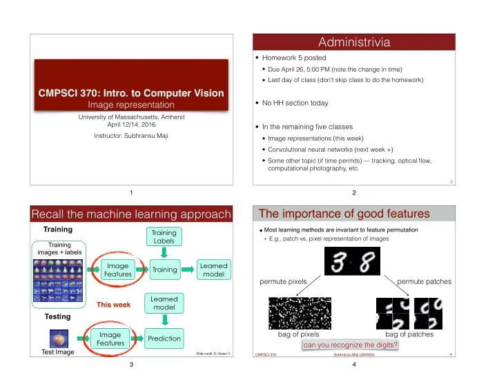2 1 2 The importance of good features Recall the machine learning approach Training Most learning methods are invariant to feature permutation Training ‣ E.g., patch vs. pixel representation of images Labels Training images + labels Image Learned Training Features model permute pixels permute patches Learned This week model Testing Image bag of pixels bag of patches Prediction Features can you recognize the digits? Test Image Slide credit: D. Hoiem 3 CMPSCI 370 Subhransu Maji (UMASS) 4 3 4

The importance of good features What is a feature map? Consider matching with image patches Any transformation of an image into a new representation ‣ What could go wrong? Example: transform an image into a binary edge map template match quality image e.g., cross correlation Image source: wikipedia CMPSCI 370 Subhransu Maji (UMASS) 5 CMPSCI 370 Subhransu Maji (UMASS) 6 5 6 Feature map goals We will discuss … Introduce invariance to nuisance factors Two popular image features ‣ Illumination changes ‣ Histogram of Oriented Gradients (HOG) ‣ Small translations, rotations, scaling, shape deformations ‣ Bag of Visual Words (BoVW) Applications of these features Preserve larger scale spatial structure Image: [Fergus05] CMPSCI 370 Subhransu Maji (UMASS) 7 CMPSCI 370 Subhransu Maji (UMASS) 8 7 8

Histogram of Oriented Gradients HOG feature: basic idea Introduced by Dalal and Triggs (CVPR 2005) Divide the image into blocks An extension of the SIFT feature Compute histograms of gradients for each regions HOG properties: ‣ Preserves the overall structure of the image ‣ Provides robustness to illumination and small deformations gradient spatial magnitude and and orientation orientation binning HOG feature image Gradient norm HOG feature CMPSCI 370 Subhransu Maji (UMASS) 9 CMPSCI 370 Subhransu Maji (UMASS) 10 9 10 HOG feature: full pipeline Effect of bin-size Smaller bin-size: better spatial resolution Larger bin-size: better invariance to deformations Optimal value depends on the object category being modeled ‣ e.g. rigid vs. deformable objects additional invariance 10x10 cells 20x20 cells CMPSCI 370 Subhransu Maji (UMASS) 11 CMPSCI 370 Subhransu Maji (UMASS) 12 11 12

Template matching with HOG Multi-scale template matching p HOG feature map Template Detector response map ����� ( � , � ) = w · φ ( � , � ) Compute the HOG feature map for the image (f) Convolve the template with the feature map to get score Find peaks of the response map (non-max suppression) Image pyramid HOG feature pyramid What about multi-scale? • Compute HOG of the whole image at multiple resolutions • Score each sub-windows of the feature pyramid CMPSCI 370 Subhransu Maji (UMASS) 13 13 14 Example detections Example detections N. Dalal and B. Triggs, Histograms of Oriented Gradients for Human Detection, CVPR 2005 N. Dalal and B. Triggs, Histograms of Oriented Gradients for Human Detection, CVPR 2005 15 16 15 16

We will discuss … Bag of visual words • Origin and motivation of the “bag of words” model Two popular image features ‣ Histogram of Oriented Gradients (HOG) • Algorithm pipeline ‣ Bag of Visual Words (BoVW) • Extracting local features • Learning a dictionary — clustering using k-means • Encoding methods — hard vs. soft assignment • Spatial pooling — pyramid representations • Similarity functions and classifiers Figure from Chatfield et al.,2011 18 CMPSCI 370 Subhransu Maji (UMASS) 17 17 18 Bag of features Origin 1: Texture recognition • Texture is characterized by the repetition of basic elements or textons • For stochastic textures, it is the identity of the textons, not their spatial arrangement, that matters Properties: • Spatial structure is not preserved • Invariance to large translations Compare this to the HOG feature Julesz, 1981; Cula & Dana, 2001; Leung & Malik 2001; Mori, Belongie & Malik, 2001; Schmid 2001; Varma & Zisserman, 2002, 2003; Lazebnik, Schmid & Ponce, 2003 19 20 19 20

Origin 1: Texture recognition Origin 2: Bag-of-words models • Orderless document representation: frequencies of words from a dictionary Salton & McGill (1983) histogram Universal texton dictionary Julesz, 1981; Cula & Dana, 2001; Leung & Malik 2001; Mori, Belongie & Malik, 2001; Schmid 2001; Varma & Zisserman, 2002, 2003; Lazebnik, Schmid & Ponce, 2003 21 22 21 22 Origin 2: Bag-of-words models Origin 2: Bag-of-words models • Orderless document representation: frequencies of words • Orderless document representation: frequencies of words from a dictionary Salton & McGill (1983) from a dictionary Salton & McGill (1983) US Presidential Speeches Tag Cloud 
 US Presidential Speeches Tag Cloud 
 http://chir.ag/projects/preztags/ http://chir.ag/projects/preztags/ 23 24 23 24

Origin 2: Bag-of-words models Lecture outline • Orderless document representation: frequencies of words • Origin and motivation of the “bag of words” model from a dictionary Salton & McGill (1983) • Algorithm pipeline • Extracting local features • Learning a dictionary — clustering using k-means • Encoding methods — hard vs. soft assignment • Spatial pooling — pyramid representations • Similarity functions and classifiers US Presidential Speeches Tag Cloud 
 http://chir.ag/projects/preztags/ Figure from Chatfield et al.,2011 25 26 25 26 Local feature extraction Local feature extraction • Regular grid or interest regions Compute descriptor Normalize patch Detect patches Choices of descriptor: • SIFT • The patch itself corner detector • … Slide credit: Josef Sivic 28 27 27 28

Local feature extraction Lecture outline • Origin and motivation of the “bag of words” model • Algorithm pipeline … • Extracting local features • Learning a dictionary — clustering using k-means • Encoding methods — hard vs. soft assignment • Spatial pooling — pyramid representations • Similarity functions and classifiers Extract features from many images Slide credit: Josef Sivic Figure from Chatfield et al.,2011 30 29 30 Learning a dictionary Learning a dictionary … … Clustering Slide credit: Josef Sivic Slide credit: Josef Sivic 31 31 32

Learning a dictionary Clustering Basic idea: group together similar instances Visual vocabulary Example: 2D points … Clustering Slide credit: Josef Sivic CMPSCI 370 Subhransu Maji (UMASS) 34 33 34 Clustering Clustering algorithms Basic idea: group together similar instances Simple clustering: organize elements into k groups Example: 2D points ‣ K-means ‣ Mean shift ‣ Spectral clustering Hierarchical clustering: organize What could similar mean? elements into a hierarchy ‣ One option: small Euclidean distance (squared) ‣ Bottom up - agglomerative dist( x , y ) = || x − y || 2 ‣ Top down - divisive 2 ‣ Clustering results are crucially dependent on the measure of similarity (or distance) between points to be clustered CMPSCI 370 Subhransu Maji (UMASS) 35 CMPSCI 370 Subhransu Maji (UMASS) 36 35 36

Clustering examples Clustering examples Image segmentation: break up the image into similar regions Clustering news articles image credit: Berkeley segmentation benchmark CMPSCI 370 Subhransu Maji (UMASS) 37 CMPSCI 370 Subhransu Maji (UMASS) 38 37 38 Clustering examples Clustering examples Clustering queries Clustering people by space and time image credit: Pilho Kim CMPSCI 370 Subhransu Maji (UMASS) 39 CMPSCI 370 Subhransu Maji (UMASS) 40 39 40

Clustering using k-means Lloyd’s algorithm for k-means Given (x 1 , x 2 , …, x n ) partition the n observations into k ( ≤ n) sets Initialize k centers by picking k points randomly among all the points S = {S 1 , S 2 , …, S k } so as to minimize the within-cluster sum of Repeat till convergence (or max iterations) squared distances ‣ Assign each point to the nearest center (assignment step) k The objective is to minimize: X X || x − µ i || 2 arg min S k i =1 x ∈ S i X X || x − µ i || 2 arg min ‣ Estimate the mean of each group (update step) S i =1 x ∈ S i k X X || x − µ i || 2 arg min cluster center S i =1 x ∈ S i CMPSCI 370 Subhransu Maji (UMASS) 41 CMPSCI 370 Subhransu Maji (UMASS) 42 41 42 k-means in action k-means for image segmentation K=2 K=3 Grouping pixels based on intensity similarity feature space: intensity value (1D) http://simplystatistics.org/2014/02/18/k-means-clustering-in-a-gif/ CMPSCI 370 Subhransu Maji (UMASS) 43 CMPSCI 370 Subhransu Maji (UMASS) 44 43 44