Administrivia Finals (everyone) Thursday, May 5, 1-3pm, Hasbrouck - PowerPoint PPT Presentation

Administrivia • Finals (everyone) • Thursday, May 5, 1-3pm, Hasbrouck 113 — Final exam • Tuesday, May 3, 4-5pm, Location: TBD (Review?) • Syllabus includes everything taught after and including SIFT CMPSCI 370: Intro. to Computer Vision features. Lectures March 03 onwards. Deep learning University of Massachusetts, Amherst April 19/21, 2016 • Honors section Instructor: Subhransu Maji • Tuesday, April 26, 4-5pm — 20 min presentation • Friday, May 6, midnight — writeup of 4-6 pages 2 Overview Traditional Recognition Approach • Shallow vs. deep architectures • Background • Traditional neural networks • Inspiration from neuroscience Image/ Object 
 Hand-designed 
 Trainable 
 • Video Stages of CNN architecture Class feature extraction classifier Pixels • Visualizing CNNs • State-of-the-art results • Packages • Features are not learned • Trainable classifier is often generic (e.g. SVM) Many slides are by Rob Fergus and S. Lazebnik 3 4

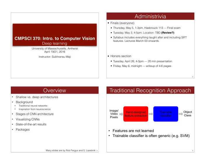
Traditional Recognition Approach What about learning the features? • Features are key to recent progress in recognition • Learn a feature hierarchy all the way from pixels to classifier • Multitude of hand-designed features currently in use • Each layer extracts features from the output of previous layer • SIFT, HOG, …………. • Train all layers jointly • Where next? Better classifiers? Or keep building more features? Image/ Simple 
 Video Layer 1 Layer 2 Layer 3 Classifier Pixels Felzenszwalb, Girshick, 
 Yan & Huang 
 McAllester and Ramanan, PAMI 2007 (Winner of PASCAL 2010 classification competition) 5 6 “Shallow” vs. “deep” architectures Artificial neural networks Traditional recognition: “Shallow” architecture Image/ Hand-designed 
 Trainable 
 Object 
 Video feature extraction classifier Class Pixels Deep learning: “Deep” architecture image credit wikipedia Image/ Simple Object • Artificial neural network is a group of interconnected nodes Video Layer 1 Layer N … classifier Class Pixels • Circles here represent artificial “neurons” • Note the directed arrows (denoting the flow of information) 7 8

Inspiration: Neuron cells Hubel/Wiesel Architecture • D. Hubel and T. Wiesel (1959, 1962, Nobel Prize 1981) • Visual cortex consists of a hierarchy of simple, complex, and hyper-complex cells Source http://en.wikipedia.org/wiki/Neuron 9 10 Perceptron: a single neuron Example: Spam Basic unit of computation Imagine 3 features (spam is “positive” class): ‣ Input are feature values ‣ free (number of occurrences of “free”) ‣ Each feature has a weight ‣ money (number of occurrences of “money”) ‣ Sum in the activation ‣ BIAS (intercept, always has value 1) w T x email x w X w i x i = w T x activation( w , x ) = i w 1 x 1 If the activation is: w 2 ‣ > b, output class 1 Σ > b x 2 ‣ otherwise, output class 2 w T x > 0 → SPAM!! x → ( x , 1) w 3 x 3 w T x + b → ( w , b ) T ( x , 1) CMPSCI 689 Subhransu Maji (UMASS) 11 /19 CMPSCI 689 Subhransu Maji (UMASS) 12 /19

Geometry of the perceptron Two-layer network architecture In the space of feature vectors y = v T h ‣ examples are points (in D dimensions) ‣ an weight vector is a hyperplane (a D-1 dimensional object) Non-linearity is important ‣ One side corresponds to y=+1 link function ‣ Other side corresponds to y=-1 Perceptrons are also called as linear classifiers h i = f ( w T i x ) w tanh( x ) = 1 − e − 2 x w T x = 0 1 + e − 2 x CMPSCI 689 Subhransu Maji (UMASS) 13 /19 CMPSCI 370 Subhransu Maji (UMASS) 14 The XOR function Training ANNs Can a single neuron learn the XOR function? Exercise: come up with the parameters of a two layer network with two hidden units that computes the XOR function ‣ Here is a table for the XOR function “Chain rule” of gradient d f ( g (x))/dx = (d f /d g )(d g /dx) we know the desired output • Back-propagate the gradients to match the outputs • Were too impractical till computers became faster http://page.mi.fu-berlin.de/rojas/neural/chapter/K7.pdf 16 CMPSCI 370 Subhransu Maji (UMASS) 15

Issues with ANNs ANNs for vision • In the 1990s and early 2000s, simpler and faster learning methods such as linear classifiers, nearest neighbor classifiers, and decision trees were favored over ANNs. • Why? • Need many layers to learn good features — many parameters need to be learned • Needs vast amounts of training data (related to the earlier point) • Training using gradient descent is slow, get stuck in local minima The neocognitron , by Fukushima (1980) (But he didn’t propose a way to learn these models) 17 18 Convolutional Neural Networks Convolutional Neural Networks • • Feed-forward feature extraction: Neural network with specialized connectivity structure 1. Convolve input with learned filters Feature maps • 2. Stack multiple stages of feature Non-linearity 3. Spatial pooling extractors Normalization 4. Normalization • Higher stages compute more • Supervised training of convolutional 
 global, more invariant features filters by back-propagating 
 • Classification layer at the end Spatial pooling classification error Non-linearity Convolution (Learned) Y. LeCun, L. Bottou, Y. Bengio, and P. Haffner, Gradient-based learning applied to document Input Image recognition, Proceedings of the IEEE 86(11): 2278–2324, 1998. 19 20

1. Convolution 2. Non-Linearity • • Per-element (independent) Dependencies are local • Translation invariance • Options: • Few parameters (filter weights) • Tanh • Stride can be greater than 1 
 • Sigmoid: 1/(1+exp(-x)) • Rectified linear unit (ReLU) (faster, less memory) Simplifies backpropagation - - Makes learning faster - Avoids saturation issues 
 à Preferred option . . . Input Feature Map 21 22 3. Spatial Pooling 4. Normalization • • Sum or max Within or across feature maps • • Before or after spatial pooling Non-overlapping / overlapping regions • Role of pooling: • Invariance to small transformations • Larger receptive fields (see more of input) Max Feature Maps 
 Feature Maps After Contrast Normalization Sum 23 24

Compare: SIFT Descriptor CNN successes • Handwritten text/digits Lowe 
 [IJCV 2004] • MNIST (0.17% error [Ciresan et al. 2011]) Image Apply 
 • Arabic & Chinese [Ciresan et al. 2012] Pixels oriented filters • Simpler recognition benchmarks • CIFAR-10 (9.3% error [Wan et al. 2013]) • Traffic sign recognition Spatial pool 0.56% error vs 1.16% for humans 
 - [Ciresan et al. 2011] (Sum) • But until recently, less good at more 
 complex datasets Feature 
 Normalize to • Caltech-101/256 (few training examples) Vector unit length 25 26 ImageNet Challenge 2012 ImageNet Challenge 2012 [Deng et al. CVPR 2009] • Similar framework to LeCun’98 but: • Bigger model (7 hidden layers, 650,000 units, 60,000,000 params) • More data (10 6 vs. 10 3 images) GPU implementation (50x speedup over CPU) • • Trained on two GPUs for a week • Better regularization for training (DropOut) • 14+ million labeled images, 20k classes • Images gathered from Internet • Human labels via Amazon Turk • The challenge: 1.2 million training images, 1000 classes A. Krizhevsky, I. Sutskever, and G. Hinton, ImageNet Classification with Deep Convolutional A. Krizhevsky, I. Sutskever, and G. Hinton, ImageNet Classification with Deep Convolutional Neural Networks, NIPS 2012 Neural Networks, NIPS 2012 27 28

ImageNet Challenge 2012 Visualizing CNNs Krizhevsky et al. -- 16.4% error (top-5) Next best (SIFT + Fisher vectors) – 26.2% error 30 22.5 Top-5 error rate % 15 7.5 0 SuperVision ISI Oxford INRIA Amsterdam M. Zeiler and R. Fergus, Visualizing and Understanding Convolutional Networks, 
 arXiv preprint, 2013 29 30 Layer 1 Filters Layer 1: Top-9 Patches • Patches from validation images that give maximal activation of a given feature map Similar to the filter banks used for texture recognition 31 CMPSCI 370 Subhransu Maji (UMASS) 32

Layer 2: Top-9 Patches Layer 3: Top-9 Patches CMPSCI 370 Subhransu Maji (UMASS) 33 CMPSCI 370 Subhransu Maji (UMASS) 34 Layer 4: Top-9 Patches Layer 5: Top-9 Patches CMPSCI 370 Subhransu Maji (UMASS) 35 CMPSCI 370 Subhransu Maji (UMASS) 36

Evolution of Features During Training Evolution of Features During Training 37 38 Occlusion Experiment • Mask parts of input with occluding square • Monitor output (class probability) Total activation in most 
 Other activations from 
 active 5 th layer feature map same feature map 40 39

Total activation in most 
 Other activations from 
 p(True class) Most probable class active 5 th layer feature map same feature map 41 42 Total activation in most 
 Other activations from 
 p(True class) Most probable class active 5 th layer feature map same feature map 43 44