Administrivia Homework 2 due today CMPSCI 370: Intro to Computer - - PowerPoint PPT Presentation

CMPSCI 370: Intro to Computer Vision

Image processing: #4 Corner detection

University of Massachusetts, Amherst February 22/24, 2015 Instructor: Subhransu Maji 1

• Homework 2 due today
• Homework 3 will be posted later this week
• will be due March 10
• No class or honors section next Tuesday, 3/1
• I am out of town to attend a CVPR program committee meeting
• Honors section will meet today

Administrivia

2

2

• Edge detection
• Derivative filters
• Corner detection [today]
• What are corners?
• Why detect corners?
• Harris corner detector

Overview

3

E = q G2

x + G2 y

image

3

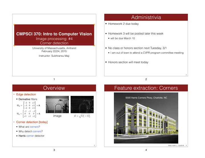
Feature extraction: Corners

4

9300 Harris Corners Pkwy, Charlotte, NC

Slide credit: L. Lazebnik

4

• Motivation: panorama stitching
• We have two images – how do we combine them?

Why extract features?

5 Slide credit: L. Lazebnik

5

• Motivation: panorama stitching
• We have two images – how do we combine them?

Why extract features?

6

Step 1: extract features Step 2: match features

Slide credit: L. Lazebnik

6

• Motivation: panorama stitching
• We have two images – how do we combine them?

Why extract features?

7

Step 1: extract features Step 2: match features Step 3: align images

Slide credit: L. Lazebnik

7

• Repeatability
• The same feature can be found in several images despite geometric and photometric

transformations

• Saliency
• Each feature is distinctive
• Compactness and efficiency
• Many fewer features than image pixels
• Locality
• A feature occupies a relatively small area of the image; robust to clutter and occlusion

Characteristics of good features

8 Slide credit: L. Lazebnik

8

Feature points are used for:

• Image alignment
• 3D reconstruction
• Motion tracking
• Robot navigation
• Indexing and database retrieval
• Object recognition

Applications

9 Slide credit: L. Lazebnik

9

A hard feature matching problem

10

NASA Mars Rover images

10

NASA Mars Rover images with SIFT feature matches
 Figure by Noah Snavely

Answer below (look for tiny colored squares…)

11

11

• A corner is the intersection of two edges
• We know how to detect edges
• Corner detector v1
• Detect edges in images (Gx and Gy)
• Find places where both Gx and Gy are high

Corner detection: Attempt one

12

• Problem: this also finds slanted edges

12

• We should easily recognize the corners by looking through

a small window

• Shifting a window in any direction should give a large

change in intensity at a corner

Corner detection: Attempt two

13

“edge”:
 no change along the edge direction “corner”:
 significant change in all directions “flat” region:
 no change in all directions

13

• We should easily recognize the corners by looking through

a small window

• Shifting a window in any direction should give a large

change in intensity at a corner

Corner detection: Attempt two

14

“edge”:
 no change along the edge direction “corner”:
 significant change in all directions “flat” region:
 no change in all directions

14

• Implementing a corner detector
• Fix the size of the patch (window size)
• What happens if the window is too small? or too large?
• Consider eight directions, and measure how much does a patch

change in each direction for each location of the image

Corner detection: Attempt two

15

15

• One way to measure change is to consider the sum of

squared-differences. Thus, the change for a shift u, v and for an image window W is

Corner detection: details

16

E(u, v) = X

(x,y)∈W

[I(x + u, y + v) − I(x, y)]2

I(x, y) W(u, v) W

16

• Assume for now that the window size W is one pixel
• How can we compute E(u,v) for every pixel in the image?
• As an example consider E(1, 0), i.e. image shifted by one

pixel to the right. This can be computed as convolution with f and squaring the result,

Corner detection: details

17

E(u, v) = X

(x,y)∈W

[I(x + u, y + v) − I(x, y)]2

D(1, 0) = I ∗   −1 1   Matlab: imfilter(I, f, ‘same’) f

17

• Generalize to any window size W
• Given D(1,0) for each pixel, how can you compute the sum-
• f-squared-differences within a window?
• Answer: filter the output with a box kernel
• Better version: Convolve with a Gaussian kernel
• More emphasis on the center than the boundary for each window

Corner detection: details

18

EdgeScore(1, 0) = f W

box ∗ D(1, 0)2

18

• Corner detector v2
• Input: image I, window size W
• Output: corner score for each pixel
• Initialize: score = zeros(size(I))
• for u = -1:1 % horizontal shifts
• for v = -1:1 % vertical shifts
• imdiff = imfilter(I, f(u,v), ‘same’); % compute difference
• score = score + imfilter(imdiff.^2, ones(W), ‘same’); % weighted

squared difference

• Here, f(u,v) is the filter to compute difference between a pixel and

another shifted by (u,v)

Corner detection: algorithm

19

19

Corner score example

20

W = 5 W = 10

σ = 2 σ = 5 Gaussian filter Box filter image

20

• Threshold the score (user specified)
• Find the peaks of responses: a pixel is a peak if it has a

higher value than all the pixels in its neighborhood

• 4 connectivity, 8 connectivity, etc
• The Matlab command imregionalmax computes a binary

image which is 1 at the peak and 0 elsewhere

• Note that there can be multiple pixels at each peak. We can

simply pick one for each connected component.

Corner detection: remaining steps

21

peak

21

• Corner detector v2
• Input: image I, window size W, threshold T
• Output: corner score for each pixel
• Initialize: score = zeros(size(I))
• for u = -1:1 % horizontal shifts
• for v = -1:1 % vertical shifts
• imdiff = imfilter(I, f(u,v), ‘same’); % compute difference
• score = score + imfilter(imdiff.^2, ones(W), ‘same’); % weighted

squared difference

• score = nms(score > T); % perform non-maximum suppression
• locs = find(score > 0); % indices of the corners
• [cy, cx] = ind2sub(size(score), lots)); % their x, y locations

Corner detection: complete algorithm

22

22

• The algorithm presented is the basis for the Harris corner

detector

• One weakness is that we only considered only 8 directions

for computing the differences. Why not 16? or 32?

• The Harris detector generalizes this to “all” directions
• More directions improve performance
• Can be thought of the limit of the earlier algorithm as the number
• f directions approach infinity!
• However, it does this without explicitly enumerating directions. To

understand how we need some math.

Corner detection: summary

23

23

Corner detection: Mathematics

24

Recall that the change in appearance of window W for the shift [u,v]:

E(3,2)

E(u, v) = X

(x,y)∈W

[I(x + u, y + v) − I(x, y)]2

I(x, y) E(u, v)

24

Corner detection: Mathematics

25

E(0,0)

E(u, v) = X

(x,y)∈W

[I(x + u, y + v) − I(x, y)]2

I(x, y) E(u, v)

Recall that the change in appearance of window W for the shift [u,v]:

25

Corner detection: Mathematics

26

We want to find out how this function behaves for small shifts

E(u, v) = X

(x,y)∈W

[I(x + u, y + v) − I(x, y)]2

E(u, v)

Recall that the change in appearance of window W for the shift [u,v]:

26

• First-order Taylor approximation for small motions [u, v]:
• Let’s plug this into E(u,v)

Corner detection: Mathematics

27

I(x + u, y + v) = I(x, y) + Ixu + Iyv

E(u, v) = X

(x,y)∈W

[I(x + u, y + v) I(x, y)]2 ' X

(x,y)∈W

[I(x, y) + Ixu + Iyv I(x, y)]2 = X

(x,y)∈W

[Ixu + Iyv]2 = X

(x,y)∈W

⇥ I2

xu2 + IxIyuv + IyIxuv + I2 yv2⇤

27

Corner Detection: Mathematics

28

The quadratic approximation can be written as where M is a second moment matrix computed from image derivatives:

[ ]

! " # $ % & ≈ v u M v u v u E ) , (

! ! ! " # $ $ $ % & =

∑ ∑ ∑ ∑

y x y y x y x y x y x y x x

I I I I I I M

, 2 , , , 2

(the sums are over all the pixels in the window W)

28

• The surface E(u,v) is locally approximated by a

quadratic form. Let’s try to understand its shape.

• Specifically, in which directions 


does it have the smallest/greatest
 change?

Interpreting the second moment matrix

29

! " # $ % & ≈ v u M v u v u E ] [ ) , (

E(u, v)

! ! ! " # $ $ $ % & =

∑ ∑ ∑ ∑

y x y y x y x y x y x y x x

I I I I I I M

, 2 , , , 2

29

First, consider the axis-aligned case (gradients are either horizontal or vertical) If either a or b is close to 0, then this is not a corner, so look for locations where both are large.

Interpreting the second moment matrix

30

! " # $ % & = b a

! ! ! " # $ $ $ % & =

∑ ∑ ∑ ∑

y x y y x y x y x y x y x x

I I I I I I M

, 2 , , , 2

30

Consider a horizontal “slice” of E(u, v):

Interpreting the second moment matrix

31

This is the equation of an ellipse. const ] [ = ! " # $ % & v u M v u

! " # $ % & = b a

31

const ] [ = ! " # $ % & v u M v u Consider a horizontal “slice” of E(u, v):

Interpreting the second moment matrix

32

This is the equation of an ellipse. R R M ! " # $ % & =

− 2 1 1

λ λ The axis lengths of the ellipse are determined by the eigenvalues and the orientation is determined by R

direction of the slowest change direction of the fastest change

(λmax)-1/2 (λmin)-1/2 Diagonalization of M:

32

Visualization of second moment matrices

33

33

Visualization of second moment matrices

34

34

Interpreting the eigenvalues

35

λ1 λ2 “Corner”
 λ1 and λ2 are large,


λ1 ~ λ2;


E increases in all

directions

λ1 and λ2 are small;
 E is almost constant

in all directions

“Edge” 
 λ1 >> λ2 “Edge” 
 λ2 >> λ1 “Flat” region

Classification of image points using eigenvalues of M:

35

Corner response function

36

“Corner”
 R > 0 “Edge” 
 R < 0 “Edge” 
 R < 0 “Flat” region |R| small

2 2 1 2 1 2

) ( ) ( trace ) det( λ λ α λ λ α + − = − = M M R

α: constant (0.04 to 0.06)

λ2 λ1

36

• 1. Compute partial derivatives at each pixel
• 2. Compute second moment matrix M in a Gaussian window

around each pixel:

The Harris corner detector

37

C.Harris and M.Stephens. “A Combined Corner and Edge Detector.” Proceedings of the 4th Alvey Vision Conference: pages 147—151, 1988.

! ! ! " # $ $ $ % & =

∑ ∑ ∑ ∑

y x y y x y x y x y x y x x

I y x w I I y x w I I y x w I y x w M

, 2 , , , 2

) , ( ) , ( ) , ( ) , (

37

• 1. Compute partial derivatives at each pixel
• 2. Compute second moment matrix M in a Gaussian window

around each pixel

• 3. Compute corner response function R

The Harris corner detector

38

C.Harris and M.Stephens. “A Combined Corner and Edge Detector.” Proceedings of the 4th Alvey Vision Conference: pages 147—151, 1988.

38

Harris Detector: Steps

39

39

Harris Detector: Steps

40

Compute corner response R

40

• 1. Compute partial derivatives at each pixel
• 2. Compute second moment matrix M in a Gaussian window

around each pixel

• 3. Compute corner response function R
• 4. Threshold R
• 5. Find local maxima of response function (non-maximum

suppression)

The Harris corner detector

41

C.Harris and M.Stephens. “A Combined Corner and Edge Detector.” Proceedings of the 4th Alvey Vision Conference: pages 147—151, 1988.

41

Harris Detector: Steps

42

Find points with large corner response: R > threshold

42

Harris Detector: Steps

43

Take only the points of local maxima of R

43

Harris Detector: Steps

44

44

• We want corner locations to be invariant to photometric

transformations and covariant to geometric transformations

• Invariance: image is transformed and corner locations do not change
• Covariance: if we have two transformed versions of the same image,

features should be detected in corresponding locations

Invariance and covariance

45

45

Image translation

46

• Derivatives and window function are shift-invariant

Corner location is covariant w.r.t. translation

46

• Original corner detector paper
• C.Harris and M.Stephens, “A Combined Corner and Edge Detector.”

Proceedings of the 4th Alvey Vision Conference,1988

• Other corner functions
• Can you think of other that work for finding corners?

Further thoughts and readings…

47

f(λ1, λ2)

47