Adapting the PPMstar Code to run on GPUs Paul Woodward Laboratory - - PowerPoint PPT Presentation

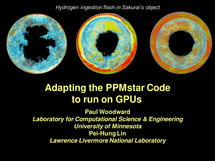
Hydrogen ingestion flash in Sakurai’s object

Adapting the PPMstar Code to run on GPUs

Paul Woodward Laboratory for Computational Science & Engineering University of Minnesota Pei-Hung Lin Lawrence Livermore National Laboratory

Time evolution of the radial location of the He-shell flash convection zone based on the 1-D stellar evolution model of

• Herwig. Time is set to 0 at the peak of the He-burning luminosity. Dots represent individual time steps. Lagrangian

lines at different mass fractions are shown. The convection zone grows both in radius and in mass fraction over the 2- year interval shown. Our simulation is performed at about time 0.2 yr on this slide.

Here we see the central 0.2% of the simulation domain, convection cells as large as about a fifth of the entire convection zone are seen by this time.

PPM simulation

• f VLTP star

helium shell flash convection

• n a 15363

grid. Note the trains of small vortices containing entrained, stable gas being drawn down into the convection zone.

Slice of 3-D Domain t = 400 min. |∇×u|

Here we see the upper boundary of the convection zone above the helium burning shell, looking from the center of the star outward. The blue descending plumes trace out the convection cells

PPM simulation

• f VLTP star

helium shell flash convection

• n a 15363

grid. Note the trains of small vortices containing entrained, stable gas being drawn down into the convection zone.

Half of 3-D Domain t = 400 min. FVH+He

Energy release from burning ingested hydrogen is shown as the dark purple and yellow/red flame.

Here we see the upper boundary of the convection zone above the helium burning shell, looking from the center of the star outward. The blue descending plumes trace out the convection cells

PPM simulation

• f AGB star

helium shell flash convection

• n a 15363

grid. Note the trains of small vortices containing entrained, stable gas being drawn down into the convection zone.

Top Half of 3-D Domain t = 400 min. FVH+He

Energy release from burning ingested hydrogen is shown as the dark purple and yellow/red flame.

Sakurai’s Object H-ingestion simulation on Blue Waters machine in Jan., 2014, on a grid of 15363 cells. We see a hemisphere and make only mixtures

• f entrained

hydrogen-rich gas with gas of the helium shell flash convection zone

• visible. The energy

release rate from burning ingested H is shown in very dark blue, yellow, and white. t = 650 min. Burning is now

• ccurring at

a larger number

• f loca-

tions at the same time.

Sakurai’s Object H-ingestion simulation on Blue Waters machine in Jan., 2014, on a grid of 15363 cells. We see a hemisphere and make only mixtures

• f entrained

hydrogen-rich gas with gas of the helium shell flash convection zone

• visible. The energy

release rate from burning ingested H is shown in very dark blue, yellow, and white. t = 1188 min. The burning front has now reached the antipode, where violent, localized energy release drives the

• scill-

ation back to its

• rigin-

al site. GOSH = Global Oscillation

• f Shell

Hydrogen ingestion.

Sakurai’s Object H-ingestion simulation on Blue Waters machine in Jan., 2014, on a grid of 15363 cells. We see a hemisphere and make only mixtures

• f entrained

hydrogen-rich gas with gas of the helium shell flash convection zone

• visible. The energy

release rate from burning ingested H is shown in very dark blue, yellow, and white. t = 1200 min. The GOSH is indeed global. This flow has a 1-D average, but it is by no means a 1-D phen-

• men-
• n.

Blue Waters makes it possi- ble to see the GOSH in its full 3-D complexity.

Sakurai’s Object H-ingestion simulation on Blue Waters machine in Jan., 2014, on a grid of 15363 cells. We see a hemisphere and make only mixtures

• f entrained

hydrogen-rich gas with gas of the helium shell flash convection zone

• visible. The energy

release rate from burning ingested H is shown in very dark blue, yellow, and white. t = 1212 min. Once the GOSH quiets down, after about a day in the life

• f this

star, we can be well justi- fied in carry- ing our descrip- tion of the star forward with a 1-D stellar evolution code, suitably modified.

Sakurai’s Object H-ingestion simulation on Blue Waters machine in Jan., 2014, on a grid of 15363 cells. We see a hemisphere and make only mixtures

• f entrained

hydrogen-rich gas with gas of the helium shell flash convection zone

• visible. The energy

release rate from burning ingested H is shown in very dark blue, yellow, and white. t = 1225 min.

Sakurai’s Object H-ingestion simulation on Blue Waters machine in Jan., 2014, on a grid of 15363 cells. We see a hemisphere and make only mixtures

• f entrained

hydrogen-rich gas with gas of the helium shell flash convection zone

• visible. The energy

release rate from burning ingested H is shown in very dark blue, yellow, and white. t = 1238 min.

Sakurai’s Object H-ingestion simulation on Blue Waters machine in Mar., 2015, on a grid of 15363 cells. We see a hemisphere and make only mixtures

• f entrained

hydrogen-rich gas with gas of the helium shell flash convection zone visible. Vorticity in a thin slice shows convection penetrating into upper, H-enriched layer. t = dump 1406 1261 min.

Sakurai’s Object H-ingestion simulation on Blue Waters machine in Mar., 2015, on a grid of 15363 cells. We see a hemisphere and make only mixtures

• f entrained

hydrogen-rich gas with gas of the helium shell flash convection zone visible. Vorticity in a thin slice 90° from previous one shows that H-ingestion has reached an entirely new level. t = dump 1800

Sakurai’s Object H-ingestion simulation on Blue Waters machine in Mar., 2015, on a grid of 15363 cells. We see a hemisphere and make only mixtures

• f entrained

hydrogen-rich gas with gas of the helium shell flash convection zone visible. A thin slice taken at 90° from the previous view shows sloshing on equipotentials producing mixing. t = dump 1800 1442 min.

Pei-Hung and I volunteered, the rest of the team passed:

• 1. Goal: Can we tap into the potential of the GPUs?
• a. Previous tries with Fermi GPU failed.

Performance was about 50% of 1 CPU of the day.

• b. Kepler is better.

1) More adders and multipliers (not necessary) 2) More registers per thread (a liberation) 3) Peak so high that even 5% of it would be great. c. I had good experience moving PPB phase space advection to the GPU in Zurich in summer of 2014.

• 2. Impossible unless:
• a. Compress on-chip work space to 32 KB (= L1 cache).
• b. Never call syncthreads.

c. Prefetch data in globs of 128 words only, with each such fetch overlapped with computation.

• d. Do significant amount of unnecessary computation in
• rder to save storage space on chip. 10% extra flops.

Features of PPMstar related to High Performance & Scalability:

• 1. Briquette data structure.
• a. Dimension DD(4,4,2,16,2,nbqs)
• b. Dimension indxbq(4,0:nbqx+1,0:nbqy+1,0:nbqz+1,8)

c. Building AMR version.

• d. DD is bunch of briquette records, 43 cells, 16 variables.
• e. indxbq is a look-up table – indirect addressing of bqs.
• 2. Bizarre & difficult Fortran code expression, but readable.
• a. Updates an entire pencil of briquettes in 1-D sweep.
• b. Pipelined update of pair of grid planes of 4×4×2 cells.

c. 91 KB of instructions for 1100 flops/cell, 29 KB workspace.

• 3. CFDbuilder automatic code translator.
• a. Truly wonderful but does not apply to GPU friendly version.
• 4. Within big loop, pattern repeated 4 times per traversal:
• a. Receive a glob of 128 words landing in on-chip cache.
• b. Prefetch next glob of 128 words.

c. Launch write-back of 128 words.

• d. Compute what can while data trickles onto and off of chip.

The computation proceeds along a sequence of briquettes at same grid level. In the on-chip cache workspace, we have many short segments

• f grid planes, each

holding one variable and none > 5 planes. These briquettes are in transit between main memory and the cache. In the cache, we unpack arriving briquettes into

• ur temporary segments,

and we pack results into updated briquettes.

What did we have to do to get to the GPU?

• 1. Everything we did for CELL processor and Intel MIC.
• a. No problem, did that already. Have code translator.
• 2. New feats:

1) Redefine basic data structure to fetch half-briquettes. 2) Process 2 rather than 1 grid plane of 4×4 cells at once. New, but related, pipelining transformation. 3) Rearrange subroutines to consume data in globs and to minimize data that must persist from glob to glob. 4) Prefetch data in globs rather than whole bq at once. 5) Essentially do register allocation. Totally unreasonable. I swore that I would never do this. Using subroutine stacks (or {} in CUDA) to do this is not allowed, because it will force stalls on data transfers.

• a. Could a tool do this for you?

1) Of course. 2) Pei-Hung Lin will write it in ROSE if his management allows it. It would help if you signed a petition.

Asessing the Potential Benefit:

• 1. On the dual CPU node of Blue Waters:
• a. Achieve about 70 Gflop/s, or just 12% of peak.
• b. To accomplish this now (in new GPU-oriented code):

1) Prefetch off-chip data 128 words ahead of need. 2) Process two 16-cell “grid planes” at a time in fully vectorized mode on SIMD engine. 3) Pipeline computation to eliminate redundant work (not all of it) and to reuse cached data. 4) Compress on-chip workspace to 29 KB. 5) Instructions are 91 KB. c. Why is performance only 12% of peak? 1) Each core has tiny SIMD register file – way too small. 2) Bandwidth in and out of register file is way too low. 3) Cannot evict temporary results to L1 and read in new

• perands from L1 in time to keep SIMD engine busy.

4) About 80% of time is register spilling, apparently. 5) The chip could be redesigned to fix all this, of course.

Asessing the Potential Benefit 2:

• 1. On the Kepler K20 GPU with 6-D PPB:
• a. Achieve about 150 Gflop/s, or just 4.3% of peak, on PPB

phase space fluid advection. (28 words in+out, 281 flops)

• b. To accomplish this:

1) Prefetch off-chip data 128 words ahead of need. 2) Process one 32-cell “grid plane” at a time in fully vectorized mode on SIMD engine. 3) Pipeline computation to eliminate all redundant work and to reuse cached data maximally. 4) Compress on-chip workspace to 16 KB. 5) Instructions are relatively few & NO logic. c. Why is performance only 4.3% of peak? 1) Each core is waiting on arrival of data 85% of time. 2) Bandwidth onto and off of chip is too low. 3) Cannot overlap waits on data with computation by

• ther threads just like this – no room for them.

4) Chip redesign could fix all these limitations, of course.

Asessing the Potential Benefit 3:

• 1. On the Kepler K20 GPU with PPMstar:
• a. Achieve about 121 Gflop/s, or just 3.4% of peak.
• b. To accomplish this 1.68× speedup over BW node:

1) Prefetch off-chip data 128 words ahead of need. 2) Process two 16-cell “grid planes” at a time in fully vectorized mode on SIMD engine. 3) Pipeline computation to eliminate most redundant work and to reuse cached data a lot. 4) Compress on-chip workspace to 20.6 KB. 5) Instructions are still 91 KB, we can’t help that. c. Why is performance only 3.4% of peak? 1) Each core is waiting on data to emerge from a very long processing pipes, with only 8 threads/core. 2) Compiler apparently cannot find any other

• perands to throw into the pipe until these emerge.

3) Cannot fit enough simultaneous threads onto chip. 4) Chip redesign could fix all this, of course.

Asessing the Potential Benefit 4:

• 1. How are others doing with CFD on GPUs?
• a. WRF microphysics runs at twice our speed in Gflop/s.

1) It accounts for only 25% of the code’s running time. 2) After years, whole code has not been moved to GPU.

• b. ASUCA weather code in Japan.

1) 51 Gflop/s per K20x GPU while running on 4108 GPUs. 2) Full implementation of code, but only half our speed. c. Swiss team at ETH Zurich using Stella DSL. 1) Parareal advection diffusion, VERY simple. 2) 4.5x speedup over single Sandy Bridge CPU 3) But what is 1 ??? 4) Use GNU compiler. (We find GNU Fortran is worst.) 5) Get only 5x speedup from running 8 threads on the 8

• cores. (We get 10x from 16 threads on 8 cores).

6) Code seems memory bandwidth limited on CPU. (Ours is not, so they screwed up on CPU, apparently.)

• 2. We seem to be doing as well as or better than these others.

Tentative Conclusion:

• 1. K20 GPU likely not worth trouble for CFD w/o translator.
• a. Too much work for too little benefit.
• b. Restructured code much more difficult to maintain.

c. You could do it if you had to, but it is really hard.

• d. Potential chip design changes that might help:

1) Prefetch more than 128 words at a time. 2) Build arithmetical pipes that complete in 5 or 6 clocks, like everyone else does. 3) Build a compiler that will try to rearrange instruction order to keep pipe full. 4) Put a reasonable instruction cache onto the chip. 5) Add simple instructions to realign data in just one

• clock. This cannot be hard. Standard since 1973.

6) Produce a more reasonable balance between on- chip data storage capacity and arithmetical units.

• e. These things could happen.

1) They will never happen if we do not ask for them.

Tentative Conclusion:

• 1. K80 GPU better, but not better enough.
• a. Our performance increases to 216 Gflop/s.
• b. What made this 79% improvement?

1) More replicas of code per core enabled. 2) However, each replica still allowed max of only 32 KB. 3) Coding effort still immense. 4) Still always waiting for results to pop out of pipes. c. 216 Gflops is triple present BW node performance. 1) But BW nodes old and K80 is new. 2) Dual Sandy Bridge node gives 114 Gflop/s & is old. 3) Dual Haswell node likely to at least match K80 perf.

• 2. Nvidia is trying, but not hard enough.
• a. Why can’t I have fewer threads with more on-chip data?
• b. Other chips and compilers can keep pipes full;

what is Nvidia’s problem with this? c. Why can’t I prefetch 4 KB all at once without stalling?

• d. With 28 MB data on chip, why can’t I fit 91 KB of instructions?

GPU design is for up to 64 simultaneous threads per core:

• 1. 64 threads all fetching contiguous data covers latency.
• a. This would be great if we cared about latency.
• b. We can prefetch, and hence latency is irrelevant.

1) We simply PLAN our computation. 2) We pack the data we need in contiguous records. 3) Address records, not words, indirectly at no cost. 4) We have lots to do while data arrives. c. Nvidia does not permit a single thread to prefetch more than a trivial amount of off-chip data. 1) Disastrous loss of performance, or coding handstands. 2) By demanding at least 8 threads per core, we are denied the space to stash arriving data even if we were allowed to prefetch it.

• d. For CFD, we are better off with 2 threads/core, not 64.
• 2. 64 threads doing identical operations keeps long pipes full.
• a. This would be great if we had 64 threads.
• b. There is not enough space for the data 64 threads require.

Why can’t we compute Nvidia’s way; what is our problem?

• 1. Nvidia’s way requires order of magnitude more data traffic
• nto and off of the chip.
• a. The chip does not offer enough bandwidth for this.
• b. Even if it did, it is a bad solution, with huge power cost.

1) Moving the data on the chip is much more efficient than moving it onto and off of the chip. 2) Would have to get rid of some arithmetical units. 3) Why have arithmetical units only LinPack can use? 4) We have to stop quoting or reading LinPack numbers. c. Nvidia offers useless cache space on the chip. 1) We update our data, we don’t just read it. 2) Practically no “shared memory” space per thread.

• 2. Nvidia GPUs get better on each generation.
• a. They will eventually be powerful and easy to use for CFD.
• b. I might see the day, but it is not today.

c. Fixes to chip that would greatly improve my code’s performance do not seem difficult or expensive at all.