SLIDE 1 2002 HST Calibration Workshop Space Telescope Science Institute, 2002
- S. Arribas, A. Koekemoer, and B. Whitmore, eds.
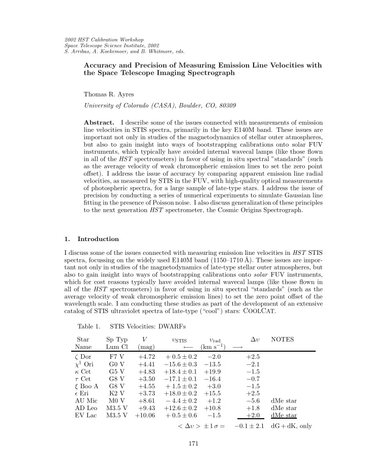
Accuracy and Precision of Measuring Emission Line Velocities with the Space Telescope Imaging Spectrograph
Thomas R. Ayres University of Colorado (CASA), Boulder, CO, 80309 Abstract. I describe some of the issues connected with measurements of emission line velocities in STIS spectra, primarily in the key E140M band. These issues are important not only in studies of the magnetodynamics of stellar outer atmospheres, but also to gain insight into ways of bootstrapping calibrations onto solar FUV instruments, which typically have avoided internal wavecal lamps (like those flown in all of the HST spectrometers) in favor of using in situ spectral ”standards” (such as the average velocity of weak chromospheric emission lines to set the zero point
- ffset). I address the issue of accuracy by comparing apparent emission line radial
velocities, as measured by STIS in the FUV, with high-quality optical measurements
- f photospheric spectra, for a large sample of late-type stars. I address the issue of
precision by conducting a series of numerical experiments to simulate Gaussian line fitting in the presence of Poisson noise. I also discuss generalization of these principles to the next generation HST spectrometer, the Cosmic Origins Spectrograph. 1. Introduction I discuss some of the issues connected with measuring emission line velocities in HST STIS spectra, focussing on the widely used E140M band (1150–1710 ˚ A). These issues are impor- tant not only in studies of the magnetodynamics of late-type stellar outer atmospheres, but also to gain insight into ways of bootstrapping calibrations onto solar FUV instruments, which for cost reasons typically have avoided internal wavecal lamps (like those flown in all of the HST spectrometers) in favor of using in situ spectral “standards” (such as the average velocity of weak chromospheric emission lines) to set the zero point offset of the wavelength scale. I am conducting these studies as part of the development of an extensive catalog of STIS ultraviolet spectra of late-type (“cool”) stars: COOLCAT. Table 1. STIS Velocities: DWARFs Star Sp Typ V υSTIS υrad ∆υ NOTES Name Lum Cl (mag) ← − (km s−1) − → ζ Dor F7 V +4.72 + 0.5 ± 0.2 −2.0 +2.5 χ1 Ori G0 V +4.41 −15.6 ± 0.3 −13.5 −2.1 κ Cet G5 V +4.83 +18.4 ± 0.1 +19.9 −1.5 τ Cet G8 V +3.50 −17.1 ± 0.1 −16.4 −0.7 ξ Boo A G8 V +4.55 + 1.5 ± 0.2 +3.0 −1.5 ǫ Eri K2 V +3.73 +18.0 ± 0.2 +15.5 +2.5 AU Mic M0 V +8.61 − 4.4 ± 0.2 +1.2 −5.6 dMe star AD Leo M3.5 V +9.43 +12.6 ± 0.2 +10.8 +1.8 dMe star EV Lac M3.5 V +10.06 + 0.5 ± 0.6 −1.5 +2.0 dMe star < ∆υ > ± 1 σ = −0.1 ± 2.1 dG + dK, only 171
SLIDE 2
172 Ayres Figure 1. Sample measurements, using a semi-autonomous Gaussian fitting al- gorithm, of selected C I emissions in an E140M spectrum of the K dwarf ǫ Eridani. Table 2. STIS Velocities: GIANTs and SUPERGIANTs Star Sp Typ V υSTIS υrad ∆υ NOTES Name Lum Cl (mag) ← − (km s−1) − → υ Peg F8 III +4.40 − 6.2 ± 1.1 −11.1 +4.9 high υ sini 31 Com G0 III +4.94 + 1.1 ± 1.8 −1.4 +2.5 high υ sini 35 Cnc G0 III +6.58 +42.4 ± 2.3 +36.0 +6.4 high υ sini HR 9024 G1 III +5.90 − 2.6 ± 0.3 +0.7 −3.3 high υ sini 24 UMa G4 III +4.57 −26.8 ± 0.3 −27.2 +0.4 µ Vel G5 III +2.72 + 6.8 ± 0.3 +6.2 +0.6 ι Cap G8 III +4.30 +12.1 ± 0.2 +11.5 +0.6 β Cet K0 III +2.04 +13.4 ± 0.2 +13.0 +0.4 α Boo K1.5 III −0.04 − 4.3 ± 0.2 −5.2 +0.9 α Tau K5 III +0.85 +54.2 ± 0.2 +54.3 −0.1 α TrA K2 II +1.92 − 3.4 ± 0.3 −3.3 −0.1 β Aqr G0 Ib +2.91 + 7.1 ± 0.3 +6.5 +0.6 broad-lined β Cam G1 Ib +4.03 − 0.8 ± 0.6 −1.7 +0.9 broad-lined ǫ Gem G8 Ib +3.02 + 6.8 ± 1.0 +9.9 −3.1 broad-lined < ∆υ > ± 1 σ = +0.4 ± 0.4 narrow-lined, only
SLIDE 3
STIS Emission Line Velocities 173 Figure 2. Summary of velocity measurements in the sample. The target features all are narrow chromospheric lines. The solar-type star α Cen A shows that such features fall to better than 1 km s−1 of the expected stellar radial velocity (in this case based on the well-determined orbit of the α Cen system). 2. Accuracy I addressed the issue of accuracy by comparing apparent emission line velocities, as measured by STIS in the FUV, with optical determinations of radial velocities, for a sample of nearly thirty late-type stars. Figure 1 depicts the semi-autonomous measuring procedure for a group of C I lines in a representative K-type dwarf. Figure 2 summarizes average emission- line velocities of the targets, based on selected narrow low-excitation chromospheric emission lines, ostensibly free of blends and optical depth effects. Tables 1 and 2 compare the STIS velocities (±1 s.e. [standard error] of the mean) with υrads from SIMBAD (the radial velocity material, unfortunately, is somewhat inhomogeneous) for the two dozen or so single (or wide binary) stars of the sample. The absolute velocity accuracy of a typical STIS pointing on a bright late-type star, based on the standard deviations, appears to be better than ±2 km s−1, with an uncertain contribution due to the optical υrads themselves.
SLIDE 4 174 Ayres Figure 3. Simulation of Gaussian fitting process for emission features governed by photon statistics (on a negligible background, in this case). The distribution functions (lower three panels) were obtained from the results of 105, or so, trials at each of several S/N levels (top panel illustrates representative line profiles). “x” is the wavelength displacement in pixels, and “stn100” is a measure of the S/N relative to the N = 100 counts case. The “normalized” quantities on the abscissa allow a scale-independent comparison of the distribution functions for different FWHM
- cases. Here, a FWHM= 2 pix simulation is shown. The dot-dashed horizontal
lines mark the probability of a (two-sided) 1 σ deviation. The lower horizontal lines indicate 2 σ (darker) and 3 σ (lighter) deviations.
SLIDE 5
STIS Emission Line Velocities 175 3. Precision I addressed the issue of precision by examining the internal consistency of the emission line measurements within the spectrum of a given star: see, again, Figures 1 and 2, Tables 1 and 2. The internal consistency of line positions appears to be extremely good, limited largely by the photon statistics of the measurements themselves. I routinely am seeing sub-km s−1 standard deviations in typical cool star emission spectra. These two exercises rely upon reasonable assessments of the errors incurred in fitting narrow emission lines with, say, a least-squares Gaussian algorithm. I have re-examined this question by conducting a series of numerical experiments to simulate Gaussian line fitting in the presence of Poisson noise: see Figure 3. These simulations lead to a series of scaling laws to describe estimated 1 σ , 2 σ, and 3 σ two-sided confidence intervals for the key Gaussian parameters—centroid wavelength λ0, full-width at half maximum intensity
FWHM, and integrated line flux fL—as a function of the S/N of the flux measurement (i.e.,
√ N for counting statistics). Complete results will appear in a future publication. Acknowledgments. Supported by HST archive research grant AR–09550.01–A.