A spool pattern tool for circular braiding J.H. van Ravenhorst* and - - PDF document

18TH INTERNATIONAL CONFERENCE ON COMPOSITE MATERIALS

Introduction Circular Braiding is a composite material preform manufacturing process that is used to manufacture bi- and triaxial braids. It provides a fast fiber lay- down due to the simultaneous fiber deposition. The highly interlaced structure of braids enables

• verbraiding of complex shaped mandrels. Braiding

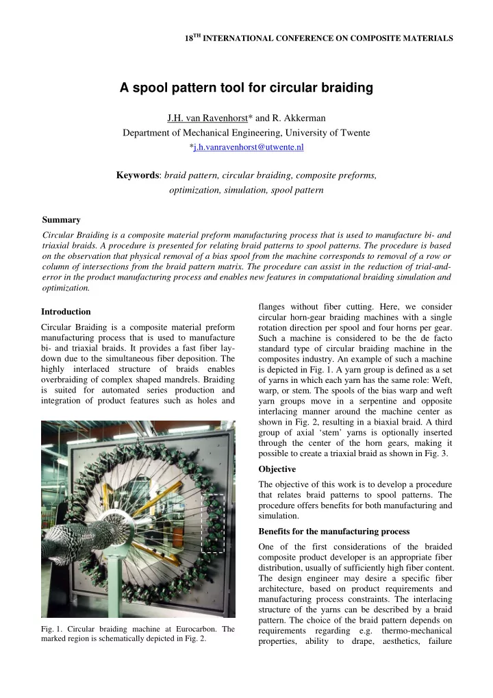
is suited for automated series production and integration of product features such as holes and flanges without fiber cutting. Here, we consider circular horn-gear braiding machines with a single rotation direction per spool and four horns per gear. Such a machine is considered to be the de facto standard type of circular braiding machine in the composites industry. An example of such a machine is depicted in Fig. 1. A yarn group is defined as a set

• f yarns in which each yarn has the same role: Weft,

warp, or stem. The spools of the bias warp and weft yarn groups move in a serpentine and opposite interlacing manner around the machine center as shown in Fig. 2, resulting in a biaxial braid. A third group of axial ‘stem’ yarns is optionally inserted through the center of the horn gears, making it possible to create a triaxial braid as shown in Fig. 3. Objective The objective of this work is to develop a procedure that relates braid patterns to spool patterns. The procedure offers benefits for both manufacturing and simulation. Benefits for the manufacturing process One of the first considerations of the braided composite product developer is an appropriate fiber distribution, usually of sufficiently high fiber content. The design engineer may desire a specific fiber architecture, based on product requirements and manufacturing process constraints. The interlacing structure of the yarns can be described by a braid

• pattern. The choice of the braid pattern depends on

requirements regarding e.g. thermo-mechanical properties, ability to drape, aesthetics, failure

A spool pattern tool for circular braiding

J.H. van Ravenhorst* and R. Akkerman Department of Mechanical Engineering, University of Twente

*j.h.vanravenhorst@utwente.nl

Keywords: braid pattern, circular braiding, composite preforms,

• ptimization, simulation, spool pattern

Summary Circular Braiding is a composite material preform manufacturing process that is used to manufacture bi- and triaxial braids. A procedure is presented for relating braid patterns to spool patterns. The procedure is based

• n the observation that physical removal of a bias spool from the machine corresponds to removal of a row or

column of intersections from the braid pattern matrix. The procedure can assist in the reduction of trial-and- error in the product manufacturing process and enables new features in computational braiding simulation and

• ptimization.
• Fig. 1. Circular braiding machine at Eurocarbon. The

marked region is schematically depicted in Fig. 2.

mechanisms and braiding process limitations. The most common biaxial braids are 2/2 twill, plain and 3/3 twill, also known as a ‘regular’, ‘diamond’ and ‘Hercules’ braids, respectively. Many other braids, as well as non-crimp fabric (NCF) architectures are possible as well. The braid pattern is used to determine the setup of the braiding machine for

• manufacturing. This is often done by the machine
• perator.

The construction of a braiding machine with four horns per gear allows it to drive a maximum of two bias carriers per gear. Half of the horns must be left vacant to allow simultaneous inter-gear transfer of the carriers. A carrier can be vacant or occupied by assignment of a spool. Hence, the amount of spools does not necessarily equal the amount of carriers. For each yarn group, the arrangement of spools over the carriers is defined as the spool pattern. The spool pattern depends, amongst others, on the desired braid pattern and mandrel dimensions. The machine construction puts a limit on the number of available braid patterns and generally only allows a single braid pattern per braiding run. Incorrect assignment of spools to carriers can lead to problems like an incorrect braid pattern, unexpected areas with a low degree of coverage, or the absence

• f interlacement altogether, potentially leading to

fabric disintegration upon handling [1], [2]. Therefore an a-priori relation between spool pattern and resulting braid pattern is preferred. Use of the relation prevents a time consuming trial-and-error process of finding the correct spool pattern. Benefits for simulation and optimization Use of computational braiding simulation and

• ptimization for arbitrary mandrels intends to reduce

lead-time and cost related to engineering, physical testing and over-dimensioning, assess ‘what-if’ scenarios, derive new design rules and output braiding machine CNC data. Features of such tools may involve the topology of the interlaced structure

• f a braid. The topology is determined by the spool

pattern, given the start points of the yarn paths. Therefore a well defined spool pattern is required. Another benefit of such a-priori knowledge is a means of checking the topological validity of the virtual braid. An example will be given later in this paper. Analysis Circular braiding can be regarded as tubular

• weaving. In contrast to weaving, however, the

weft (O) and warp (X) yarns are deposited

• simultaneously. Both techniques yield periodic
• fabrics. The smallest repetitive element for a

mesoscopic representation of periodic fabric is defined as a repeat. A repeat element size is determined by the number of weft and warp yarns or nr,X and nr,O, respectively. The subscript r refers to a

• repeat. The intersections of a weave pattern repeat

can be schematically represented by the ‘linear method’, drawing a line and intersections for each yarn,

• r

‘canvas method’ using a matrix

• representation. Biaxial braids are elaborated first

using the canvas method with indicated yarn direction. Biaxial spool patterns A machine having two occupied bias carriers per gear is defined as a full machine. It yields a 2/2 twill biaxial braid with a 4 by 4 repeat size. The repeat is depicted in Fig. 4 using the canvas method. It is possible to extend the matrix to include all spools of

• Fig. 2. Schematic carrier paths and initial positions for the

region indicated in Fig. 1. Carriers are denoted with weft (O) and warp (X). Stem yarns, indicated by (S), emerge from the gear centers.

• Fig. 3. Triaxial braid.

a full machine. The number of rows and columns then equals the number of weft and warp group carriers, indicated by nc,O, and nc,X, respectively. The subscript c refers to carriers. Generally, nc,O = nc,X = nc. The key observation here is that physical removal of a weft or warp spool from a carrier on a full machine corresponds to removing its row or column, respectively, from the full machine’s braid pattern matrix, possibly yielding a new braid pattern. An example of this procedure is given in Fig. 5. For further use of this procedure a spool pattern is represented by a bit sequence or vector s

indicating

which carriers are (‘1’) or are not (‘0’) assigned a spool, starting at the group carrier number 1. In this paper, spool patterns are also described in words for ease of reading. The size of a spool pattern is defined as the length of the smallest repetitive sequence of its bits. In the example of Fig. 5, the resulting spool pattern could be expressed as e.g.

O X

s s

• = [1010] for both weft and warp yarn

groups, but the smallest repetitive sequence is [10], yielding a size of 2. Consequently, a spool pattern size that exceeds the number of carriers of its group is invalid. Given a spool pattern as input, the bias braid pattern is readily obtained. See Fig. 6 for examples where it is assumed that both bias yarn groups have the same spool pattern. As can be

• bserved from the examples, removal of spools can

affect the value of the repeat size. For Fig. 6(a) and (b), interlacement is lost, resulting in a NCF. The canvas method is not very useful to visualize a NCF because a NCF has no interlacement. Also note that, as shown in Fig. 6(c), the 3/3 twill or Hercules braid is not as structured as its 2/2 twill equivalent. Generally, the braid pattern is not invariant to bit pattern rotation. This is exemplified in Fig. 7. The examples also illustrate the practical consequences

• f incorrect arrangement of spools over the carriers.

When a spool pattern is given, the braid pattern is easily found using the previously described

• procedure. The inverse route involves finding a

spool pattern given the braid pattern. A valid spool pattern is uniquely defined by providing the following input parameters: The amount of available carriers per group nc, the required number of spools ns, using subscript s to refer to spools, a braid pattern and, although it might seem superfluous, a spool distribution over the carriers. The spool distribution can be homogeneous, i.e. equally spaced over the

• Fig. 4. A 2/2 twill or ‘regular’ biaxial braid pattern for a

full machine, visualized with the canvas method.

• Fig. 5. Example of spool removal. Starting with a full

machine, the braid pattern is conveniently represented by four repeats (a). Next, weft and warp spools are removed from carriers with an even ID. This is represented by removal of their corresponding rows and columns (b). This yields a plain weave or ‘diamond braid’ after compaction (c) of the matrix.

carriers, clustered, etc. Omitting one of the parameters generally yields multiple spool pattern

• solutions. The importance of spool distribution is

exemplified in the following example. Suppose that for each bias group nc = 72 and ns = 24 and that a 2/2 twill braid pattern is required. Also, suppose that the spool distribution requirement is omitted. This yields multiple spool pattern solutions like 1 of 3, 2 of 6, etc, as illustrated in Fig. 8. The 1 of 3 and 2 of 6 spool patterns are examples of homogeneous and clustered spool distributions over the carriers,

• respectively. Also, the solution space of spool

patterns can be zero. For example, a 4-harness satin braid is impossible to realize because it cannot be embedded in a full machine’s braid pattern. That is, there exists no combination of weft and warp spool patterns that yields a satin. However, the satin’s well-known merit of drapability may be insignificant due to simultaneous interlacement. In practice, the amount of carriers per group nc corresponds to the choice for a specific braiding machine. The number

• f spools ns can be determined from the mandrel

dimensions, fiber angles, yarn count, degree of coverage, etc. Using an additional spool distribution constraint, e.g. homogeneous spool distribution, an

• ptimal spool pattern can be found. This can be done

either manually, or, as suggested by the title, integrated in a software tool using straightforward

• ptimization techniques. However, this had not been

fully implemented yet. Triaxial spool patterns Addition of the axial or stem yarn (S) group increases pattern complexity. Due to its simplicity for visualization and implementation, it is desirable to use the canvas representation again. This can be achieved by turning the bias canvas pattern by 45 degrees and adding the stem yarn intersections, resulting in the braiding topology matrix T as depicted in Fig. 9. Each element contains zero or one intra-yarn-group intersection. The horizontal and vertical axes correspond to the mandrel axis and mandrel circumference, respectively. T represents a single braid period around the mandrel and can be traversed as a toroidal graph. Each intra-group bias yarn pair has two intersections in T. The ‘repeat’ size in T can be up to 2nc by 2nc. Removal of spools again corresponds to removing series

• f
• intersections. By convention, the braid is deposited

from left to right. The start condition for the braid can be represented by any curve through T in circumferential direction, but is most conveniently taken to be between the last and first column, i.e. not coinciding, but just before the first series of

• intersections. The positions of the stem yarn

intersections relative to others in T do not

• Fig. 6. Braid repeats for different spool patterns after the

spool removal procedure. Spool patterns apply to both weft and warp yarn groups. Spool pattern 1 of 4 or s

= [1000] yields a two-layered NCF (a).

2 of 4 or s

= [1100] yields a four-layered NCF (b).

3 of 6 or s

= [111000] yields a 3/3 twill or Hercules

braid (c).

• Fig. 7. Example of the effect of bit pattern rotation on

braid pattern repeats.

O

s = [1001] and

X

s = [10] yield

a plain weave repeat (left). After the rotation of bits in

O

s

• to [1100] while keeping

X

s constant, a two-layered NCF

emerges (right).

• Fig. 8. Two valid spool patterns for a 2/2 twill braid

pattern and nc = 72 and ns = 24 or one third of the machine bias spool capacity for both weft and warp

• groups. Both 1 of 3 or s

= [100] (left) and 2 of 6 or s = [110000] (right) satisfy the constraints.

necessarily correspond to their physical equivalents. Stem yarns may slide ‘through’ bias yarn intersections, altering the positions

• f

stem intersection locations in T. Other bias yarn intersections can block a stem yarn. Both cases are illustrated by Fig. 10. The blocking bias interlacement points can be easily identified in T. The inverse route for triaxial braids cannot be expressed using simple weave pattern topology and is not treated here. However, the descriptions presented here can be readily implemented as an assisting tool for use in circular braiding simulations. Example of use in simulation The macroscopic paths of the bias yarns can be calculated by kinematic simulation methods as described in e.g. [3] and [4]. A novel addition to the simulation is modeling of the axial yarns. In practice, the deposition of the axial yarns is coupled with that of the bias yarns. Hence, ideally, all yarn paths are calculated simultaneously. However, to reduce complexity and improve computational performance, it is assumed that no interaction occurs between yarns. Due to the interlacing nature of a braid's bias yarns, a modeling approach can be explored where it is assumed that the position of axial yarns is predominantly determined by the bias interlacing points. The first step in such an approach involves the calculation of the bias yarn paths and

• intersections. Next, for each axial yarn, this

information is used in combination with T to model their topological and geometric bounds and expected

• positions. The quality of this approach can be

validated experimentally. Conclusion A procedure is proposed for relating braid patterns to spool patterns. The procedure aims to reduce trial- and-error in the product manufacturing process and enables new features in computational braiding simulation and optimization. Acknowledgements The support of Agentschap NL, Eurocarbon B.V. and the National Aerospace Laboratory NLR is gratefully acknowledged. References

[1] A. Pickett, J. Sirtautas and A. Erber. Braiding simulation and prediction of mechanical properties, Applied Composite Materials, Vol. 16, pp 345-364, 2009. [2] M. Siegrist. Wirtschaftliche RTM- Prozesstechnologien für die Herstellung von CFK-

• Motorradfelgen. M.Sc. thesis, ETH Zürich, 2006.

[3] J.F.A. Kessels and R. Akkerman. Simulations of the braiding process for RTM preforms, Proceedings of TexComp 5, Leuven, Belgium, 2000. [4] R. Akkerman and B. Rodriguez. Braiding simulation and slip evaluation for arbitrary mandrel, ESAFORM-10, AIP Conference Proceedings, Vol.907, pp1074-1079, 2007.

• Fig. 9. Triaxial topology matrix T for a full machine. One

circumferential and three axial repeats are drawn.

• Fig. 10. Yarn interaction types at different bias interlacing

points from Fig. 9.