A Mechanical Model to Simulate Interactively a Bending Actuator - - PDF document

SLIDE 1

A Mechanical Model to Simulate Interactively a Bending Actuator Composed of three Parallel Bellows

• P. Joli1*, N. Seguy1, Z.Q. Feng2

1Laboratoire Systèmes Complexes, Université d'Evry, 40 rue du Pelvoux, 91020 Evry, France

e-mail: pjoli@iup.univ-evry.fr

2Laboratoire de Mécanique d'Evry, Université d'Evry, 40 rue du Pelvoux, 91020 Evry, France

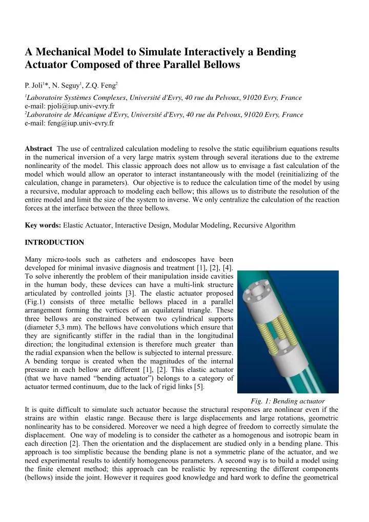
e-mail: feng@iup.univ-evry.fr Abstract The use of centralized calculation modeling to resolve the static equilibrium equations results in the numerical inversion of a very large matrix system through several iterations due to the extreme nonlinearity of the model. This classic approach does not allow us to envisage a fast calculation of the model which would allow an operator to interact instantaneously with the model (reinitializing of the calculation, change in parameters). Our objective is to reduce the calculation time of the model by using a recursive, modular approach to modeling each bellow; this allows us to distribute the resolution of the entire model and limit the size of the system to inverse. We only centralize the calculation of the reaction forces at the interface between the three bellows. Key words: Elastic Actuator, Interactive Design, Modular Modeling, Recursive Algorithm INTRODUCTION Many micro-tools such as catheters and endoscopes have been developed for minimal invasive diagnosis and treatment [1], [2], [4]. To solve inherently the problem of their manipulation inside cavities in the human body, these devices can have a multi-link structure articulated by controlled joints [3]. The elastic actuator proposed (Fig.1) consists of three metallic bellows placed in a parallel arrangement forming the vertices of an equilateral triangle. These three bellows are constrained between two cylindrical supports (diameter 5,3 mm). The bellows have convolutions which ensure that they are significantly stiffer in the radial than in the longitudinal direction; the longitudinal extension is therefore much greater than the radial expansion when the bellow is subjected to internal pressure. A bending torque is created when the magnitudes of the internal pressure in each bellow are different [1], [2]. This elastic actuator (that we have named “bending actuator”) belongs to a category of actuator termed continuum, due to the lack of rigid links [5].

• Fig. 1: Bending actuator

It is quite difficult to simulate such actuator because the structural responses are nonlinear even if the strains are within elastic range. Because there is large displacements and large rotations, geometric nonlinearity has to be considered. Moreover we need a high degree of freedom to correctly simulate the

• displacement. One way of modeling is to consider the catheter as a homogenous and isotropic beam in

each direction [2]. Then the orientation and the displacement are studied only in a bending plane. This approach is too simplistic because the bending plane is not a symmetric plane of the actuator, and we need experimental results to identify homogeneous parameters. A second way is to build a model using the finite element method; this approach can be realistic by representing the different components (bellows) inside the joint. However it requires good knowledge and hard work to define the geometrical

SLIDE 2

conditions between the different types of finite elements (1D, 2D or 3D finite element) and the computation time is too high if we want to reinitialize many times some parameters of the modeling. In this paper we present an adapted numerical modeling for our hydraulic actuator to be simulated

• interactively. The challenge is to have a software tool to build a first draft virtual prototype of the

"bending actuator" with the possibility to easily change geometrical parameters or internal pressures. In

• rder to reduce the computational time, each bellow is modeled individually as an articulated multi-body

system with elastic joints, and the relative joint coordinates are calculated by a backward formulation [6]. The elasticity parameters associated to each joint are obtained by analyzing the structural response of one bellow’s convolution by a finite element modeling. Because the modeling is geometrical non linear, the computation procedure is iterative. Since the degrees of freedom between the three bellows are not independent, we have to calculate the tangent stiffness matrix of each bellow at each iteration to formulate the geometrical constraint equations in function of reaction forces between the three bellows and the moving cylindrical support. This formulation is an extension to the geometrically nonlinear problem of the "gluing algorithm" presented in [7].

• 1. Modeling of a bellow

a) Deformation hypothesis A bellows is modelled as a set of n circular sections. The movement between two successive circular sections is defined by the combination of three elementary relative movements (2 rotations, 1 translation) (Fig. 2). If we make an analogy with the theory of beams, these circular sections represent sections of internal cohesion.

• Fig. 2. Bellows of length L modeled by n circular sections

The two rotation movements correspond to the deformation caused by a bending torque. The translation movement corresponds to the deformation caused by a tension/compression force. Given the deformations described previously (hypothesis of the model), the deformation caused by a shearing effort are disregarded. The transformation matrix from Ri-1 to Ri is: [ ]

1 i i i i i i i i i i i i i

C S P S S C C S C S S C C β β β α α β α α β α α β

−

⎡ ⎤ ⎢ ⎥ = − ⎢ ⎥ ⎢ ⎥ − ⎣ ⎦ with

( ); ( ) C Cos S Sin = = ฀ ฀ ฀ ฀

(1)

and the relative position of Ri with Ri-1 is defined by:

1

1

i

i i i

O O z δ

−

→ −

= r . The parameters of the bellows are the number of convolutions N and the step of one convolution P. The greater the number of circular sections n used in the model, the greater the accuracy of the model. However, since n must be inferior to the number of convolutions N, N should preferably be a multiple of

• n. Depending on the accuracy required, the number of degrees of freedom can be very high.

b) Static bellow model To each degree of freedom between two circular sections i-1and i, we associate a stiffness:

• To the relative translation along the axis

1 1

(0 , )

i i

z

− −

r we associate the stiffness

t

K

• 1 rotation βi around yi
• 1 rotation αi around xi-1
• 1 translation δi along zi-1

zn yn zi-1 xi-1 xi yi L ON xn z0 y0 Oi-1 Oi

SLIDE 3

• To the two relative rotation movements respectively to the axis

1

(0 , )

i i

x − r and axis (0 , )

i i

y r , we associate the stiffness

f

K .

With

;

t t f f

n n K k K k N N = =

, kt and kf are the stiffness of one convolution respectively in translation and in rotation. The length L of the bellows is defined by L= NxP (P is the convolution step). The distance between two circular sections before deformation is δ* =(N/n)xP. The static equilibrium equations of the system {section i … section n} give :

( 1) ( 1)

( )

ext i i ext n i n ext i i

R R M O OO R M

− → −

⎧ + = ⎪ ⎨ + Λ + = ⎪ ⎩ r r r r r r r

with

* ( 1) 1 ( 1) 1 ( 1)

. ( ) . .

i i i t i i i i i f i i i i f i

R z K M x K M y K δ δ α β

− − − − −

⎧ = − − ⎪ ⎪ = − ⎨ ⎪ = − ⎪ ⎩ r r r r r r (2)

{ } { }

{ }

{ } { }

( ) ; ; ; ( )

i i ext i ext i i ext i i i i ext i i i i

L X R M O M R Y T M O N Z ⎧ ⎫ ⎧ ⎫ ⎧ ⎫ ⎪ ⎪ ⎪ ⎪ ⎪ ⎪ = = = ⎨ ⎬ ⎨ ⎬ ⎨ ⎬ ⎪ ⎪ ⎪ ⎪ ⎪ ⎪ ⎩ ⎭ ⎩ ⎭ ⎩ ⎭ r r r r

( )

( )

ext i ext n i n ext

M O M O O O R

→

= + Λ r r r

which gives :

*

; ;

i i i i i i i i i i i i i i i i i f f t

M L C N S Y S Z C C X C S K K K β β α α β α β β α δ δ + + − = = = +

(3)

We note that the static model is completely explicit even though it is nonlinear from a geometrical point

• f view. First we calculate recursively the components of the tensor { }

i

T and then successively βi, αi , δi

for i varying from n to 1. But each bellow inside the actuator are not independent, the tensor { }

i

T represents reaction mechanical

effort which, as we will see later, are calculated iteratively by an incremental formulation. So we need the following differential form of (3) to update the geometrical configuration of the bellow:

1 1 1

; ;

i i i i i i i

k k k k k k

d d d α α α β β β δ δ δ

+ + +

= + = + = + and { }

{ } { }

1 k k i i i

T T dT

+ =

+

; with [ ]

1 1

i i i f i

dL d dM K dN β ⎧ ⎫ ⎪ ⎪ = ⎨ ⎬ ⎪ ⎪ ⎩ ⎭

;

1 (

i i k k k i i i i i i f f i i

dL dL E d C S dM dM K K dN dN α β β ⎧ ⎫ ⎧ ⎫ ⎡ ⎤ ⎪ ⎪ ⎪ ⎪ ⎡ ⎤ = + ⎢ ⎥ ⎨ ⎬ ⎨ ⎬ ⎣ ⎦ ⎢ ⎥ ⎪ ⎪ ⎪ ⎪ ⎣ ⎦ ⎩ ⎭ ⎩ ⎭

)

2

1 ( ( ) )

i i k k k k k k k k k k k i i i i i i i i i i i i i i i t f f f f i i

dX dL C E A S d C S S C C dY B B B dM K K K K K dZ dN β β δ α β α α β ⎧ ⎫ ⎧ ⎫ ⎡ ⎤ ⎪ ⎪ ⎪ ⎪ ⎡ ⎤ = − + − ⎢ ⎥ ⎨ ⎬ ⎨ ⎬ ⎣ ⎦ ⎢ ⎥ ⎪ ⎪ ⎪ ⎪ ⎣ ⎦ ⎩ ⎭ ⎩ ⎭

(4)

with

k k k k k k k i i i i i i i

A Z C S X C C α β α β = + ,

k k k k k k k k i i i i i i i i i

B Y C Z S C X S S α α β α β = − + ,

k k k k k i i i i i

E N C L S β β = −

• Recursive calculation of {

}

i

dT

{ } [ ] { }

1 1 i i T i i

dT L dT

− −

=

with

[ ] [ ] [ ] [ ] [ ]

1 1

1 1 1 1

( )

O O i i i

i i i T i i i i i

P L S P P

→ ⎧ ⎫ ⎨ ⎬ − ⎩ ⎭ −

− − − −

⎡ ⎤ ⎢ ⎥ = ⎢ ⎥ ⎡ ⎤ ⎣ ⎦ ⎣ ⎦

with the screw matrix

1 1

( )

O O i i i

i i

S δ δ

→ ⎧ ⎫ ⎨ ⎬ − ⎩ ⎭ −

− ⎡ ⎤ ⎢ ⎥ ⎡ ⎤ = ⎣ ⎦ ⎢ ⎥ ⎢ ⎥ ⎣ ⎦ (5)

By backward recurrence, we obtain :

[ ] [ ] [ ] [ ]

1 1 1 1... i i i n T T T T n i i n

L L L L

− − − +

= Remark: This backward recurrence can also be formalised in the following way :

[ ] [ ] [ ] [ ]

1 1 1 2 1

...

n n n i U U U U i n n i

L L L L

− − − − −

= ; with [ ] [ ]

( )

[ ] {

} { } { }

1 1 1 1

ˆ ˆ ˆ ; ;

T T i i i U T U i i i i i i i i i i i i

L L L dT dT dT dL dM dN dX dY dZ

− − − −

= = =

c) Geometrical model of a bellow in Cartesian space.

SLIDE 4

The geometrical model of a bellow in cartesian space is defined by the transformation matrix [ ]

n

R which

defines the relative orientation of the reference frame Rn with the reference frame R0 and by the vector

{ }

n

O O

→

which defines the relative position of Rn with R0. The geometrical model in Cartesian space is deduced, after having calculated the static model, from the equality :

[ ] [ ] [ ] [ ] [ ]

( )

O On

n T n n n

P L S P P

→ ⎧ ⎫ ⎨ ⎬ ⎩ ⎭

⎡ ⎤ ⎢ ⎥ = ⎢ ⎥ ⎡ ⎤ ⎣ ⎦ ⎣ ⎦ (6)

Three parameters of position and three parameters of rotation are sufficient to define the geometrical model. Parameters of position ⇒ Cartesian coordinates. {

}

{ }

)

n S

• x

O O y z χ

→

⎧ ⎫ ⎪ ⎪ = = ⎨ ⎬ ⎪ ⎪ ⎩ ⎭

Parameters of rotation ⇒ Yaw, Pitch, Roll angles [ ]

[ ] [ ] [ ]

' '' ' ' ''

( , ) ( , ) ( , )

n n n n n n n n

P Rot z Rot y Rot x φ θ ψ = r r r

[ ]

n n

C C C S S S C C S C S S P S C S S S C C S S C C S S C S C C φ θ φ θ ψ φ ψ φ θ ψ φ ψ φ θ φ θ ψ φ ψ φ θ ψ φ ψ θ θ ψ θ ψ − + ⎡ ⎤ ⎢ ⎥ = + − ⎢ ⎥ ⎢ ⎥ − ⎣ ⎦

The inverse relations are:

21 11 31 11 21 13 23 12 22

atan2( , ); atan2( , ); atan2( , ) p p p C p S p S p C p S p C p φ θ φ φ ψ φ φ φ φ = = − + = − − +

(7)

with

[ ]

11 12 13 21 22 23 31 32 23 n n

p p p P p p p p p p ⎡ ⎤ ⎢ ⎥ = ⎢ ⎥ ⎢ ⎥ ⎣ ⎦

. We note afterwards : { }

S

φ η θ ψ ⎧ ⎫ ⎪ ⎪ = ⎨ ⎬ ⎪ ⎪ ⎩ ⎭

et { } { } { }

;

S S S

χ η ⎧ ⎫ ⎪ ⎪ Λ = ⎨ ⎬ ⎪ ⎪ ⎩ ⎭

where{

}

S

Λ represents the geometrical parameters of the bellow S. d) Geometrical differential model of a bellow The small relative displacement field of Rn with R0 can be defined by the following tensor:

{ }

/ 0 T n x y z

dU du dv dw d d d = Θ Θ Θ ;

with

( / 0) ;

x n y n z n n n n n

d n d x d y d z d O O du x dv y dw z

→

Θ = Θ + Θ + Θ = + + r r r r r r r

By using the parameters, we have:

'

( / 0) ;

n n n

d n d z d y d x d O O dx x dy y dz z φ θ ψ

→

Θ = + + = + + r r r r r r r

We deduce the following relations :

[ ]{ } [ ]

1 ;

x y S S z

d S d Z d Z C S C d C C S θ η θ ψ ψ θ ψ ψ Θ − ⎧ ⎫ ⎡ ⎤ ⎪ ⎪ ⎢ ⎥ Θ = = ⎨ ⎬ ⎢ ⎥ ⎪ ⎪ ⎢ ⎥ Θ − ⎩ ⎭ ⎣ ⎦

; [ ] {

}

n S

du dv P d dw χ ⎧ ⎫ ⎪ ⎪ = ⎨ ⎬ ⎪ ⎪ ⎩ ⎭ (8)

which are equivalent to the following formulation :{

} [ ]{ }

/ 0 n S S

dU d = Π Λ

with [

] [ ] [ ]

( )

T n S

P Z ⎡ ⎤ Π = ⎢ ⎥ ⎢ ⎥ ⎣ ⎦

e) Determination of the stiffness parameters We model one convolution of a bellow (Tab. 1) by shell elements using ANSYS, a finite element

• software. In the first loading case, the convolution is subjected to a tension effort; by a series of

numerical tests we deduce the tension stiffness per convolution. In a second loading case, the convolution is subjected to a bending torque; by a series of numerical tests we deduce the flexion stiffness per convolution.

• Tab. 1. Geometrical parameters of a convolution

Exterior diameter DE (mm) Interior diameter DI (mm) Wall thickness E (mm) Convolution step P (mm) 1,60 1,02 0,013 0,25

SLIDE 5

The bellow used is made of nickel:

• Young’s modulus: E= 161115 MPa
• Poisson’s ratio: ν=0,3

After analysing numerical tests, we have obtained a tension stiffness per convolution of kt=21,145 N/mm and a bending stiffness per convolution of kf=4,8055 N.mm/rad. e) Tangential stiffness matrix of a bellow

• Tangential stiffness matrix between two circular sections

The small displacement of disc i relative to disc i-1 is defined by :

1 1 1

( / 1) ;

i i i x i y i z i i i i i i i i i i i i i i i

d i i d x d y d z d x d y d O O du x dv y dw z d z α β δ

→ − − −

Θ − = Θ + Θ + Θ = + = + + = r r r r r r r r r r

We obtain :{ } [ ]{ }

/ 1

( / 1)

i i i i

dU J i i dq

−

= −

(9)

The static model defined earlier can be written as follows: { } [ ] [ ] { } [ ]{ }

( )

1

( / 1)

t i i i i

dq D J i i dT C dT

−

= − +

with

[ ] [ ] [ ]

1 2

1 1 ; ; ( / 1) 1 ( ) 1

i i i i f f i i i f i i i i i i i i t f f f f i

C S E S K K C C D C J i i K C B C B E A B S K K K K K S α β α α β β β β β

−

− ⎡ ⎤ ⎡ ⎤ ⎡ ⎤ ⎢ ⎥ ⎢ ⎥ ⎢ ⎥ ⎢ ⎥ ⎢ ⎥ ⎢ ⎥ ⎢ ⎥ ⎢ ⎥ = = − = ⎢ ⎥ ⎢ ⎥ ⎢ ⎥ ⎢ ⎥ ⎢ ⎥ ⎢ ⎥ ⎢ ⎥ ⎢ ⎥ − ⎢ ⎥ ⎢ ⎥ ⎢ ⎥ ⎣ ⎦ ⎣ ⎦ ⎢ ⎥ ⎣ ⎦

We therefore deduce :{ }

[ ] { }

1 / 1 i i i i

dU K dT

− −

=

(10)

with [ ] [ ][ ] [ ] [ ][ ] [ ]

1 1 1

( / 1) ( / 1) ( / 1)

t i i

K J i i D J i i J i i D C

− − −

= − − + −

⇔ [ ]

1 * * / 1 i i i i

K J C

− −

⎡ ⎤ ⎡ ⎤ = + ⎣ ⎦ ⎣ ⎦

where [

]

i

K represents the tangential stiffness matrix between the circular sections i-1 and i. f) Tangential stiffness matrix of a group of n circular discs By applying the principle of the superposition of small displacements, we obtain :

{ } { } { } { }

/ 0 / 1 1/ 2 1/ 0

( ) ( ) ... ( )

n n n n n n n n

dU dU O dU O dU O

− − −

= + + +

(11)

which gives us :{

} { } [ ] { } [ ] { }

/ 0 / 1 1/ 2 1/ 0 1 1

...

n n n n n U n n U n

dU dU L dU L dU

− − − −

= + + +

By recalling the results obtained earlier in Section 1-b: [

] [ ] [ ] [ ] [ ]

1 1 1 2 ...

( )

n n n i i T U U U U T i n n i n

L L L L L

− + − −

= = we also have the following relations:

{ } [ ] { } [ ] [ ] { } [ ] [ ] { }

1 1 1 / 0 1 1 1 1 1 1

...

n n n n n U n n U n

dU K dT L K dT L K dT

− − − − − −

= + + +

{ } [ ] [ ] [ ] [ ] [ ] [ ] [ ] { }

1 1 1 1 1 / 0 1 1 1 1

( ... )

n T n n T n n T n T T T n n n n

dU K L K L L K L dT

− − − − − −

= + + +

(12)

{ } [ ] { }

1 / 0 n S n

dU K dT

−

=

where [

]

1 S

K

− is called the flexibility matrix of the bellow S.

By using the geometrical differential model, we obtain the following relations : { } [ ]{ } { } [ ] { } [ ] [ ] [ ]

1 1 / 0 1

; ;

n n S S S S

P dU d d dU Z

− − −

⎡ ⎤ ⎢ ⎥ = Π Λ ⇒ Λ = Π Π = ⎢ ⎥ ⎣ ⎦

{ } [ ]{ } [ ] [ ] [ ]

1 1

( / ) ; ( / )

S S n n S n S S

d J T dT J T K

− −

Λ = Λ Λ = Π

(13)

where [

]

( / )

S n

J T Λ

represents the flexibility matrix of the bellow relative to its geometrical parameters. g) Computation algorithm of a bellow The computation algorithm of a bellow is represented by Fig. 3. From known values at the kth iteration

• f computation { } (

1, )

k n

T i n =

, { } (

1, )

k n

q i n =

{ }

n

dT , and the new value {

}

n

dT , this algorithm calculates:

• {

} (

1, )

n

dT i n =

,{

} (

1, )

n

dq i n =

respectively the new incremental internal forces and the new incremental joint coordinates of the bellow S.

D P

SLIDE 6

• { }

1 (

1, )

k n

q i n

+

=

to update the new geometrical configuration

• {

}

1 k S +

Λ

the new geometrical parameters of the bellow S.

• [

]

1

( / )

k S n

J T

+

Λ

the new flexibility matrix of the bellow S

• Fig. 3. Algorithm flowchart of a bellow (Algorithm 1)

2 Model of the bending actuator

y x H Bellow Sa Bellow Sb Bellow Sc y x Op Onc Onb Ona

[ ] [ ]

1

,

S T n

K L

−

, , φ θ ψ

i=n ; ;

i=0

[ ] [ ] [ ] [ ] [ ] [ ]

1 1 1 1

1 1 1 1 1

( ) ; ( )

O O i i i O O i i i

i i i i i i i i i i i i i i i i i i

S S C C S S P C S P L S P P β α α β α δ β β

→ ⎧ ⎫ ⎨ ⎬ − ⎩ ⎭ − → ⎧ ⎫ ⎨ ⎬ − ⎩ ⎭ −

− − − − −

− − ⎡ ⎤ ⎢ ⎥ ⎡ ⎤ = ⎣ ⎦ ⎢ ⎥ ⎢ ⎥ ⎣ ⎦ ⎡ ⎤ ⎢ ⎥ = ⎢ ⎥ ⎡ ⎤ ⎣ ⎦ ⎣ ⎦

True

End Data :, δ*, Kt, Kf,

{ } [ ]{ }

1 i T i

dT L dT

−

=

* * * / 1 i i i i

K J C

−

⎡ ⎤ ⎡ ⎤ ⎡ ⎤ = + ⎣ ⎦ ⎣ ⎦ ⎣ ⎦

[ ]

* T T i T

X L K L ⎡ ⎤ ⎡ ⎤ ⎡ ⎤ = ⎣ ⎦ ⎣ ⎦ ⎣ ⎦

[ ] [ ] [ ]

1 1 S S

K K X

− −

= +

[ ] [ ][ ]

T T

L L L = { } [ ] { } { }

1 1

, ( / ) , , ( 1, )

S S S k k i i

J T q T i n

+ +

Λ Λ ∀ =

{ } [ ] [ ] { } [ ]{ }

1

.( ( / 1)

t i i i i

dq D J i i dT C dT

−

= − +

{ } { } { } { } { } { }

1 1

;

k k k k i i i i i i

q q dq T T dT

+ +

= + = + i=i-1

SLIDE 7

• Fig. 4. Bending actuator
• Fig. 5. Bottom view of the moving cylindrical support

Inside the bending actuator, each bellow Sa, Sb, Sc, is connected to a fixed support at one extremity and to a moving cylindrical support S at the other as shown in Figs. 4 and 5. The constraining motion of the moving extremities of the three bellows imposes the establishment of algebraic constraints for their relative positions and relative rotations. Moreover, the reaction forces applied to the moving extremities

• f the three bellows from S must verify the conditions imposed by the static equilibrium equations.

a) Static equilibrium equations

• (

)

: , , , R O x y z r r r

the fixed reference frame.

• (

)

: , , , ( , , )

i i

R O x y z i a b c = r r r , reference frames linked respectively to the fixed extremities of Sa, Sb, Sc

• ;

( 3 2 3 2 ); ( 3 2 3 2 );

a a b a c

O O H y O O H x y O O H x y

→ → →

= = − + = − r r r r r

• (

)

: , , , ( , , )

ni ni i i i

R O x y z i a b c = r r r

, reference frames linked respectively to the moving extremities of Sa, Sb, Sc. The position and orientation of each reference frame ( , , )

ni

R i a b c = is defined by {

}

Si

Λ such as : { } { } { } { }

{ } {

}

; ; ( , , )

i i i Si i i ni i i i i i

x y O O i a b c z φ χ χ η θ η ψ

→

⎧ ⎫ ⎧ ⎫ ⎧ ⎫ ⎪ ⎪ ⎪ ⎪ ⎪ ⎪ Λ = = = = = ⎨ ⎬ ⎨ ⎬ ⎨ ⎬ ⎪ ⎪ ⎩ ⎭ ⎪ ⎪ ⎪ ⎪ ⎩ ⎭ ⎩ ⎭

The static equilibrium equations of S are defined by : { } { } { } { } { }

( ) ( ) ( ) ( )

a b c

T fluide S T S S T S S T S S → − → − → − → =

(14)

We choose 0na as the reference point and Rna as the projection reference frame. Denoting ( 3 2 1.5 ); ( 3 2 1.5 )

a a a a

b H x y c H x y = − + = − r r r r r r , Eq.(14) can be rewritten by:

{ } [ ] { } [ ] { } {

}

. .

na nb nc f

T b T c T T = − − + (15) with [ ] [ ] [ ]

{ }

[ ] [ ] [ ] [ ] { } [ ]

; ( ) ( ) Id Id b c S c Id S b Id

→

⎡ ⎤ ⎡ ⎤ ⎢ ⎥ = = ⎢ ⎥ ⎡ ⎤ ⎢ ⎥ ⎡ ⎤ ⎢ ⎥ ⎢ ⎥ ⎣ ⎦ ⎢ ⎥ ⎣ ⎦ ⎣ ⎦ ⎣ ⎦ r

b) Mechanical action of fluid The hydraulic pressure inside the three bellows Sa, Sb, Sc applies a mechanical action to S defined by:

{ } { }

[ ] {

}

[ ] {

}

. .

f fa fb fc

T T b T c T = + + ; {

} { }

{ }

; ( , , );

fi fi fi i i

R T R p S z i a b c ⎧ ⎫ ⎪ ⎪ = = = ⎨ ⎬ ⎪ ⎪ ⎩ ⎭ r r r r

(16)

( , , )

i

p i a b c = represents the internal pressure of the fluid inside the bellow Si . c) Algebraic constraints for relative orientation

SLIDE 8

If the reference frame ( , , )

ni

R i a b c =

are initially all parallel to R0 and their orientation is defined

respectively by { }

T i i i

η φ θ ψ = , then we must verify that their relative orientation remains constant :{

} { } { } { } { } { } { }

0; ; ( , );

rb r r ri i a rc

i b c η η Φ ⎧ ⎫ ⎪ ⎪ Φ = Φ = Φ = − = ⎨ ⎬ Φ ⎪ ⎪ ⎩ ⎭

(17)

by derivation, we obtain:

{ } [ ]{ };

r r

d J d Φ = Λ

[ ] [ ] [ ] [ ] [ ]

r

Id Id J Id Id ⎡ ⎤ − = ⎢ ⎥ − ⎣ ⎦ ; { } { } { } { }

;

Sa Sb Sc

d d d d Λ ⎧ ⎫ ⎪ ⎪ Λ = Λ ⎨ ⎬ ⎪ ⎪ Λ ⎩ ⎭

(18)

where [

]

r

J is the jacobean matrix associated with these algebraic constraints. d) Algebraic constraints for relative position We must now verify that the two reference frames Rnb, Rnc maintain a constant relative position to Rna, we have to satisfy: ;

a b a c

O O b O O c

→ →

= = r r

{ } { } { } { } { } { } { } [ ] { }

0; ; ( , )

tb t t ti i a na tc

P i i b c χ χ Φ ⎧ ⎫ ⎪ ⎪ ⇔ Φ = Φ = Φ = − − = ⎨ ⎬ Φ ⎪ ⎪ ⎩ ⎭ r

(19)

By derivation again, we obtain the jacobean matrix [

]

t

J associated to these constraints:

{ } [ ]{ }

t t

d J d Φ = Λ with [

] [ ] [ ]

{ }

[ ] [ ] [ ] [ ] { } [ ] [ ]

( ) ( )

a na t a na

Id P S b Z Id J Id P S c Z Id ⎡ ⎤ ⎡ ⎤ − ⎣ ⎦ ⎢ ⎥ = ⎢ ⎥ − ⎡ ⎤ ⎣ ⎦ ⎣ ⎦ r r

(20)

e) The algorithm of the Bending actuator The efforts applied to the moving support must be compatible with the conditions of the static equilibrium:

{ }

{ }

[ ]{ } [ ] { }

0 . a f b c

T T b T c T = − − ⇒ {

} [ ]{ } [ ] { }

( . )

a b c

dT b dT c dT = − +

(21)

{ } { } { } { } [ ] [ ] [ ] [ ] { } { } [ ] { } { }

a b b b c c c

dT b c dT dT dT Id G dT dT dT Id dT ⎧ ⎫ ⎡ ⎤ − − ⎧ ⎫ ⎧ ⎫ ⎪ ⎪ ⎪ ⎪ ⎪ ⎪ ⎢ ⎥ = = = ⎨ ⎬ ⎨ ⎬ ⎨ ⎬ ⎢ ⎥ ⎪ ⎪ ⎪ ⎪ ⎩ ⎭ ⎩ ⎭ ⎪ ⎪ ⎢ ⎥ ⎣ ⎦ ⎩ ⎭

(22)

and must satisfy the algebraic constraints: { }

{ } { } { }

0; ;

r t

Φ ⎧ ⎫ ⎪ ⎪ Φ = Φ = ⎨ ⎬ Φ ⎪ ⎪ ⎩ ⎭ ⇒ {

} [ ]{ } [ ] [ ] [ ]

;

r t

J d J d J J ⎡ ⎤ Φ = Λ = ⎢ ⎥ ⎣ ⎦ ⇒{

} [ ] ( ) { } [ ] [ ] [ ] [ ]

( / ) / ) ; ( / ) ( / ) ( / )

Sa a Sb b Sc c

J T d J J T dT J T J T J T ⎡ ⎤ Λ ⎢ ⎥ Φ = Λ Λ = Λ ⎡ ⎤ ⎣ ⎦ ⎢ ⎥ ⎢ ⎥ Λ ⎣ ⎦

⇒{

} [ ] {

} [ ]

[ ][ ][ ]

{ }

{ } { }

1 1

; ( ( / ) ) ;

b c

dT d A dT A J J T G dT dT

− −

⎧ ⎫ ⎪ ⎪ Φ = = Λ = ⎨ ⎬ ⎪ ⎪ ⎩ ⎭ % %

(23)

The solution is obtained using the Newton-Raphston method (Fig. 6) by searching for the zero of the function { } Φ :

{ }

[ ] { } { } [ ] {

}

and

k k k

dT A dT G dT = − Φ = % %

(24)

The matrix [ ] A , [ ] G are recalculated at each kth iteration, as well as the remainder { } Φ . It is therefore necessary to call algorithm 1 for the three bellows to update their geometrical configuration and their flexibility matrix. Data :, P,N, n, kt , kf,, D

SLIDE 9

• Fig. 6. Global algorithm of bending actuator

3 Numerical results and Conclusion The proposed approach has been implemented in the LabVIEW ™ software. Many numerical tests have been performed. One of them is outlined here. In this example, the bellow is modelled with 100 circular

• sections. Only one bellow is given a pressure at each simulation. A numerical tolerance of 10-11 is

imposed on the constraints { } Φ . Tab. 2 summarises some numerical results. As we can see, the behaviour of the bending actuator seems to be coherent.

• Tab. 2: Numerical results with L=25 mm, N=100, kt =21,145 N.mm-1

kf=4,8055 N.mm.rad-1 , H=5mm, S=2,1 mm2 Algo.1 applied to Sc :

{ } [ ] [ ] { }

; ; ( / ) ; ;

Sc nc Sc c c

P J T T Λ Λ { } {

} { } { } { } { }

; ; ;

a f a b f b c f c

T T T T T T = = =

Algo.1 applied to Sb :

{ } [ ] [ ] { }

; ; ( / ) ; ;

Sb nb Sb b b

P J T T Λ Λ

*

; ; ;

t t f f

N n n P K k K k n N N δ = = = Algo.1 applied to Sa :

{ } [ ] [ ] { }

; ; ( / ) ; ;

Sa na Sa a a

P J T T Λ Λ

{ } [ ]

; ; A Φ

{ }

[ ]{ }

dT A = − Φ %

{ } [ ]{

};

dT G dT = %

True

SLIDE 10

Iteration number

a b c

p p p (N/mm2)

a b c

z z z (mm)

( ) ( ) ( ) a bc a bc a bc

φ θ ψ (rad) 4 0,2 26,60 24,75 24,75

10 10

5,410 3,810 0,249

− −

− 5 0,2 24,76 26,60 24,75 0,012 0,21 0,11 − − 5 0,2 24,76 24,75 26,60 0,012 0,21 0,12 − −

The numerical convergence is very fast. Only few iterations are necessary to obtain the solution with very good precision. However, the differential internal pressure between the three bellows should not exceed a maximum limit. This limit depends on the stiffness of the bellow (L length of the bellow, N number of convolutions, kt and kf stiffness parameters of one convolution) and on the bending moment (H cantilever distance relative to the support cylinder, S the transversal section of the bellow). If this limit is exceeded then it is necessary to implement in our algorithm an outer iterative loop to smoothly apply the internal pressure in each bellow. This is a classic problem not treated in this paper. It is also interesting to observe that, in this example, the global number of degrees of freedom is equal to 3x3x100=900 and these are coupled by 12 constraint equations. In a classic approach, we would have to inverse a large matrix (900x900). Whereas in our approach, we only need to inverse a matrix which is of always the same size (12x12). Most of the cost of the computation time is on the setting of the flexibility matrix which is linearly dependent on the number of circular discs used to model a bellow. The response time of our model is instantaneous and allows us to interact easily and quickly with the model. Further research works are being undertaken which concern the experimental validation and the comparison with finite element modelling of the bending actuator. REFERENCES [1] Joli P., François Ch., Gagarina T., Boudghène F., Modeling and process design of a new type of catheter for special endovascular treatments of abdominal aortic aneurysms, CARS2002, 849-854, Paris. [2] Thomann G., Redarce T., Bétemps M., A new Mechanism for the Orientation of the Tip of the Endoscope for the Intestinal Inspection, Proceedings of the 11 th World Congress in Mechanism and Machine Science, 2003, Tianjin (China). [3] Lim G.and al. “Multi-link active catheter snake motion” Robotica,Vol. 14, 1996 [4] Fatikow S., Rembold U., Microsystem Technology and Microrobotics, Springer-Verlag editor [5] Gravagne Ian A., Walker Ian D., Manipulability, Force and Compliance Analysis for Planar Continuum Manipulator, IEEE Transactions on Robotics and Automation, June 2002, Vol 18, N° 13, 263-273 [6] Featherstone.R. A divide-and-conquer articulated body algorithm for parallel calculation of rigid body dynamics. Part 1: Basic algorithm. International Journal of Robotic Research,Vol. 18,n° 9, pp 867-865,1999

[7]

Tseng F.-C.,. Hulbert G. M, A gluing algorithm for network-distributed dynamics simulation, Multibody System Dynamics, Vol. 6, pp. 377-396, 2003