
SLIDE 1
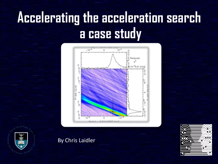
Accelerating the acceleration search a case study
By Chris Laidler
a case study By Chris Laidler Optimization cycle Assess - - PowerPoint PPT Presentation
Accelerating the acceleration search a case study By Chris Laidler Optimization cycle Assess Parallelise Test Optimise Profile le Identify the function or functions in which the application is spending most of its execution time.
By Chris Laidler
Assess Parallelise Optimise Test
–CudaDeviceSynchronize() –cudaEventSynchronize()
–cudaEventCreate(&start) –CudaEventElapsedTime()
–How, when
–CudaHostAlloc()
– cudaStreamCreate(&stream1); – Default stream - no explicit synchronization is
– cudaMemcpy()
– cudaMemcpyAsync() is a non-blocking
memcpy compute memcpy compute memcpy memcpy memcpy compute compute compute
–L1 is reserved for local memory accesses.
128 256 1 30 31 128 256 1 30 31 256 1 30 31
–Minimize Bank conflicts
divided by maximum number of warps that can run concurrently
– Registers – Shared memory
– Low occupancy kernels cannot hide memory latency
Up to 716 Hz
Up to 716 Hz
Power spectra of a 7.3 h observation of Ter 5
J1748-2446A and its harmonics J1748-2446C
Power spectra of a 7.3 h observation of Ter 5 J1748-2446A Fundamental harmonic
Power of J1748-2446A, a very strong binary pulsar. Ter A completes ∼4 orbits during the observation. The
smears the power across a number of Fourier bins.
J1748-2446A and its harmonics J1748-2446C
Power spectra of a 7.3 h observation of Ter 5 J1748-2446ae Fundamental harmonic
If we look for J1748-2446ae at ~273.33 Hz Ter AE is fairly weak and we can see there is no significant detection in the power spectra.
–Prepare (1D data)
–Multiply kernels with data –FFT –Powers
–Search fundamental –For stages ( Powers of 2, ½, ¼, 1/8, ...)
–Create –Sum with fundamental
n kernels –FFT's