
SLIDE 1
)
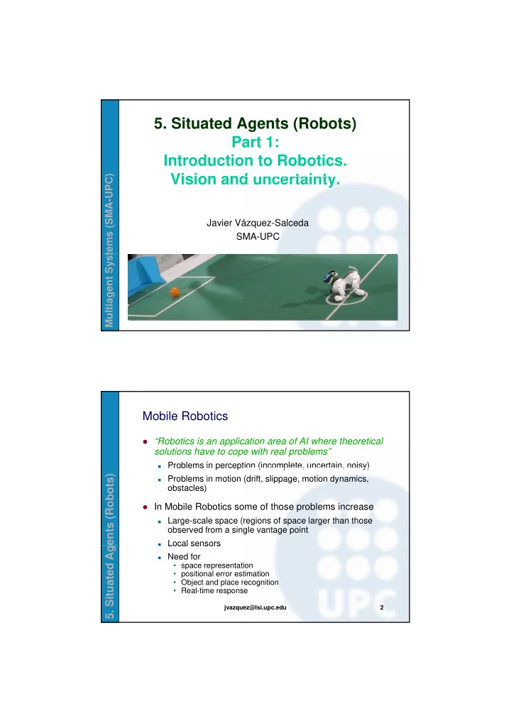
- 5. Situated Agents (Robots)
Part 1: Introduction to Robotics. Vision and uncertainty
tems (SMA-UPC
Vision and uncertainty.
Javier Vázquez-Salceda SMA-UPC
Multiagent Syst
https://kemlg.upc.edu
16/07/2012
Mobile Robotics
“Robotics is an application area of AI where theoretical
solutions have to cope with real problems”
Problems in perception (incomplete, uncertain, noisy)
ents (Robots)
p p ( p , , y)
Problems in motion (drift, slippage, motion dynamics,
- bstacles)
In Mobile Robotics some of those problems increase
Large-scale space (regions of space larger than those
- bserved from a single vantage point
Local sensors
- 5. Situated Ag
jvazquez@lsi.upc.edu 2
Local sensors Need for
- space representation
- positional error estimation
- Object and place recognition
- Real-time response