3. Random Variables Let ( , F , P ) be a probability model for an - PowerPoint PPT Presentation

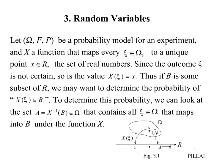
3. Random Variables Let ( Ω , F , P ) be a probability model for an experiment, and X a function that maps every to a unique ξ ∈ Ω , x ∈ ξ point the set of real numbers. Since the outcome R , is not certain, so is the value Thus if B is some ξ = X ( ) x . subset of R , we may want to determine the probability of ( ξ ∈ “ ”. To determine this probability, we can look at X ) B 1 B ξ ∈ Ω the set that contains all that maps − = ∈ Ω A X ( ) Ω into B under the function X . ξ A ( ξ X ) R x B 1 Fig. 3.1 PILLAI

1 B Obviously, if the set also belongs to the − = A X ( ) associated field F , then it is an event and the probability of A is well defined; in that case we can say 1 B − ξ ∈ = (3-1) Probabilit y of the event " X ( ) B " P ( X ( )). 1 B However, may not always belong to F for all B , thus X − ( ) creating difficulties. The notion of random variable (r.v) makes sure that the inverse mapping always results in an event so that we are able to determine the probability for any B ∈ R . Random Variable (r.v) : A finite single valued function ( ⋅ X ) that maps the set of all experimental outcomes into the Ω { } set of real numbers R is said to be a r.v, if the set ξ ξ ≤ | X ( ) x is an event for every x in R . ∈ ( F ) 2 PILLAI

Alternatively X is said to be a r.v, if where B − ∈ 1 X ( B ) F represents semi-definite intervals of the form −∞ < x ≤ { a } and all other sets that can be constructed from these sets by performing the set operations of union, intersection and negation any number of times. The Borel collection B of such subsets of R is the smallest σ -field of subsets of R that includes all semi-infinite intervals of the above form. Thus if X is a r.v, then { } { } (3-2) ξ ξ ≤ = ≤ | X ( ) x X x { } { } ? is an event for every x . What about < ≤ = a X b , X a Are they also events ? In fact with since b > X ≤ { a } a { } { } { } and are events, is an event and c X ≤ ≤ = > b X a X a { } { } hence is also an event. > ∩ ≤ = < ≤ X a X b { a X b } 3 PILLAI

  1 Thus, is an event for every n . − < ≤ a X a    n  Consequently ∞ (3-3)  1  ∩ − < ≤ = = a X a { X a }    n  = n 1 is also an event. All events have well defined probability. { } Thus the probability of the event must ξ ξ ≤ | X ( ) x depend on x . Denote { } (3-4) ξ ξ ≤ = ≥ P | X ( ) x F ( x ) 0 . X The role of the subscript X in (3-4) is only to identify the actual r.v. is said to the Probability Distribution F ( x ) X Function (PDF) associated with the r.v X . 4 PILLAI

Distribution Function : Note that a distribution function g ( x ) is nondecreasing, right-continuous and satisfies +∞ = −∞ = g ( ) 1 , g ( ) 0 , (3-5) i.e., if g ( x ) is a distribution function, then +∞ = −∞ = (i) g ( ) 1 , g ( ) 0 , x < (ii) if then ≤ x , g ( x ) g ( x ), (3-6) 1 2 1 2 and + = (iii) for all x . g ( x ) g ( x ), We need to show that defined in (3-4) satisfies all F X ( x ) properties in (3-6). In fact, for any r.v X , 5 PILLAI

{ } (3-7) (i) +∞ = ξ ξ ≤ +∞ = Ω = F X ( ) P | X ( ) P ( ) 1 { } and −∞ = ξ ξ ≤ −∞ = φ = F X ( ) P | X ( ) P ( ) 0 . (3-8) x < x , (ii) If then the subset −∞ ⊂ −∞ ( , x ) ( , x ). 1 2 1 2 { } { } , Consequently the event ξ ξ ≤ ⊂ ξ ξ ≤ | X ( ) x | X ( ) x 1 2 since implies As a result ξ ≤ ξ ≤ X ( ) x . X ( ) x 2 1 ( ) ( ) ∆ = ∆ ξ ≤ ≤ ξ ≤ = (3-9) F ( x ) P X ( ) x P X ( ) x F ( x ), X 1 1 2 X 2 implying that the probability distribution function is nonnegative and monotone nondecreasing. (iii) Let and consider the event < < < < < x x x � x x , − n n 1 2 1 { } = ξ < ξ ≤ (3-10) A | x X ( ) x . k k since { } { } { } , < ξ ≤ ∪ ξ ≤ = ξ ≤ (3-11) x X ( ) x X ( ) x X ( ) x k k 6 PILLAI

using mutually exclusive property of events we get ( ) (3-12) = < ξ ≤ = − P ( A ) P x X ( ) x F ( x ) F ( x ). k k X k X But and hence ⊂ ⊂ � A A A � , + − k 1 k k 1 ∞ (3-13) ∩ = = φ = lim A A and hence lim P ( A ) 0 . k k k → ∞ → ∞ k k = k 1 Thus = − = lim P ( A ) lim F ( x ) F ( x ) 0 . k X k X → ∞ → ∞ k k + = x But the right limit of x , and hence lim x k , → ∞ k (3-14) + = F ( x ) F ( x ), X X i.e., is right-continuous, justifying all properties of a F X ( x ) distribution function. 7 PILLAI

Additional Properties of a PDF (iv) If for some then = ≤ (3-15) 0 = x , F X ( x ) 0 , x x . F X ( x ) 0 0 0 { } ( ) This follows, since implies ξ ≤ = ξ ≤ = X ( ) x F X ( x ) P X ( ) x 0 0 0 0 { } is the null set, and for any will be a subset ≤ ξ ≤ x x , X ( ) x 0 of the null set. { } (3-16) (v) ξ > = − P X ( ) x 1 F ( x ). X { } { } We have and since the two events ξ ≤ ∪ ξ > = Ω X ( ) x X ( ) x , are mutually exclusive, (16) follows. { } (vi) (3-17) < ξ ≤ = − > P x X ( ) x F ( x ) F ( x ), x x . 1 2 X 2 X 1 2 1 { } The events and are mutually < ξ ≤ ξ ≤ { x X ( ) x } X ( ) x 1 2 1 { } . exclusive and their union represents the event ξ ≤ X ( ) x 2 8 PILLAI

( ) (vii) ξ = = − − (3-18) P X ( ) x F ( x ) F ( x ). X X Let and From (3-17) x = = − ε ε > x . x x , 0 , 2 1 { } − ε < ξ ≤ = − − ε lim P x X ( ) x F ( x ) lim F ( x ), (3-19) X X ε → ε → 0 0 or { } (3-20) ξ = = − − P X ( ) x F ( x ) F ( x ). X X + x → According to (3-14), the limit of as F X ( x ), x F X ( x ) 0 0 from the right always exists and equals However the F X ( x ). 0 − left limit value need not equal Thus F X ( x ) F X ( x ) F X ( x ). 0 0 need not be continuous from the left. At a discontinuity point of the distribution, the left and right limits are different, and from (3-20) { } ξ = = − − > (3-21) P X ( ) x F ( x ) F ( x ) 0 . 0 X 0 X 0 9 PILLAI

Thus the only discontinuities of a distribution function F X ( x ) are of the jump type, and occur at points where (3-21) is x 0 satisfied. These points can always be enumerated as a sequence, and moreover they are at most countable in number. Example 3.1: X is a r.v such that Find ξ = ξ ∈ Ω F X ( x ). X ( ) c , . { } { } , Solution: For so that and < ξ ≤ = φ = x c , X ( ) x F X ( x ) 0 , { } for so that (Fig.3.2) = > ξ ≤ = Ω F X ( x ) 1 . x c , X ( ) x , F X ( x ) 1 x c Fig. 3.2 { } Example 3.2: Toss a coin. Suppose the r.v X is Ω = H , T . such that Find F X ( x ). = = X ( T ) 0 , X ( H ) 1 . 10 PILLAI

{ } { } , Solution: For so that < ξ ≤ = φ = x 0 , X ( ) x F X ( x ) 0 . { } { } { } ≤ < ξ ≤ = = = − 0 x 1 , X ( ) x T , so that F ( x ) P T 1 p , X { } { } ≥ ξ ≤ = = Ω = x 1 , X ( ) x H , T , so that F ( x ) 1 . (Fig. 3.3) X F X ( x ) 1 q x 1 Fig.3.3 • X is said to be a continuous-type r.v if its distribution function is continuous. In that case for − = F ( x ) F ( x ) F X ( x ) X X { } all x , and from (3-21) we get = x = P X 0 . •If is constant except for a finite number of jump F X ( x ) discontinuities(piece-wise constant; step-type), then X is said to be a discrete-type r.v. If is such a discontinuity x i point, then from (3-21) { } (3-22) 11 − = = = − p P X x F ( x ) F ( x ). i i X i X i PILLAI