11/11/2014 Chapter 22 INFERENCES ABOUT MEANS 1 SAMPLING - - PDF document

11/11/2014 1

INFERENCES ABOUT MEANS

Chapter 22

1

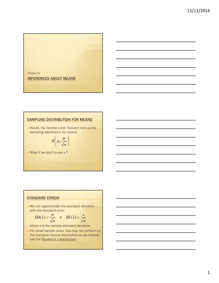
SAMPLING DISTRIBUTION FOR MEANS

 Recall, the Central Limit Theorem told us the

sampling distribution for means

 What if we don’t know σ ?

      n N  ,

2

STANDARD ERROR

 We can approximate the standard deviation

with the standard error: where s is the sample standard deviation

 For small sample sizes, this may not conform to

the standard normal distribution so we instead use the Student’s t-distribution

n s y SE n y SD    ) ( ) ( 

3

11/11/2014 2

STUDENT’S T-DISTRIBUTION

 The t-distribution is different for different sample

sizes

 It has the same general symmetric bell-shape as a

normal curve, but reflects greater variability (wider)

 Mean t = 0  Standard deviation varies with sample size, but is

greater than 1

 As n (sample size) gets larger, the t-distribution

gets closer to the standard normal distribution

4

Retrieved from http://jpkc.njmu.edu.cn/course/tongjixue/file/jxzy/ybzzSD/images/fig14-2_0.jpg, March 29, 2010.

5

Retrieved from http://www.vosesoftware.com/ModelRiskHelp/images/13/image20.gif, March 29, 2010.

6

11/11/2014 3

DEGREES OF FREEDOM

 The number of degrees of freedom (df) for a

single data set is the number of sample values that can vary after certain restrictions have been imposed on all data values

 For this application, df = n - 1

7

SAMPLING DISTRIBUTION FOR MEANS When the conditions are met, the standardized sample mean follows a Student’s t-model with n – 1 degrees

• f freedom.

We estimate the standard error with

 

y t SE y   

 

s SE y n 

8

ASSUMPTIONS AND CONDITIONS

 Independence assumption

 Randomization  10% condition

 Normal population assumption

 Nearly normal condition: The data come from a

distribution that is unimodal and symmetric.

Check this condition by making a histogram or Normal

probability plot.

9

11/11/2014 4

ONE-SAMPLE T-INTERVAL

 When the conditions are met, we are ready to find the

confidence interval for the population mean, μ.

 The confidence interval is

where the standard error of the mean is

 The critical value depends on the particular confidence level,

C, that you specify and on the number of degrees of freedom, n – 1, which we get from the sample size.

 

1 n

y t SE y

 

 

1

*

n

t 

 

s SE y n 

10

ONE-SAMPLE T-TEST FOR THE MEAN

 The conditions for the one-sample t-test for the mean are the

same as for the one-sample t-interval.

 We test the hypothesis H0:  = 0 using the statistic  The standard error of the sample mean is  When the conditions are met and the null hypothesis is true,

this statistic follows a Student’s t model with n – 1 df. We use that model to obtain a P-value.

 

1 n

y t SE y 



 

 

s SE y n 

11

TESTING HYPOTHESES ABOUT A MEAN

 The three possible choices for hypotheses are:

1.

H0: μ = μ0, HA: μ ≠ μ0

2.

H0: μ = μ0, HA: μ < μ0

3.

H0: μ = μ0, HA: μ > μ0

 μ0 is the null value

12