3 Functions of a Random Variable Consider a gas in thermal - PDF document

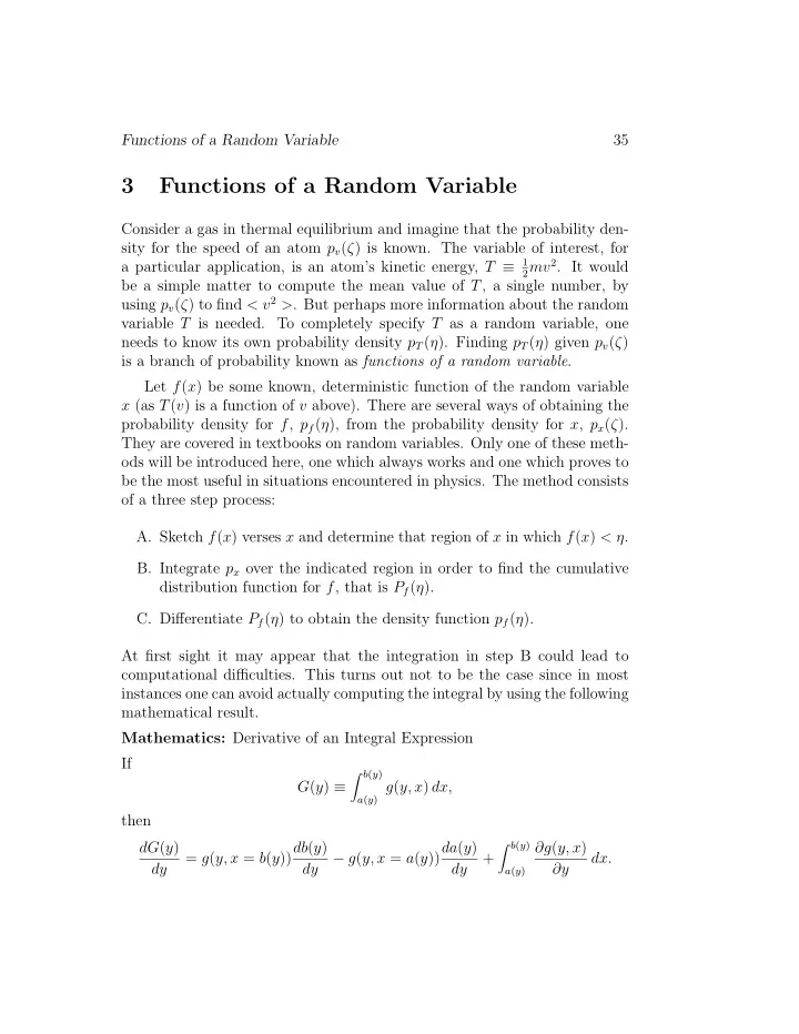
35 Functions of a Random Variable 3 Functions of a Random Variable Consider a gas in thermal equilibrium and imagine that the probability den- sity for the speed of an atom p v ( ζ ) is known. The variable of interest, for a particular application, is an atom’s kinetic energy, T ≡ 1 mv 2 . It would 2 be a simple matter to compute the mean value of T , a single number, by using p v ( ζ ) to find < v 2 > . But perhaps more information about the random variable T is needed. To completely specify T as a random variable, one needs to know its own probability density p T ( η ). Finding p T ( η ) given p v ( ζ ) is a branch of probability known as functions of a random variable . Let f ( x ) be some known, deterministic function of the random variable x (as T ( v ) is a function of v above). There are several ways of obtaining the probability density for f , p f ( η ), from the probability density for x , p x ( ζ ). They are covered in textbooks on random variables. Only one of these meth- ods will be introduced here, one which always works and one which proves to be the most useful in situations encountered in physics. The method consists of a three step process: A. Sketch f ( x ) verses x and determine that region of x in which f ( x ) < η . B. Integrate p x over the indicated region in order to find the cumulative distribution function for f , that is P f ( η ). C. Differentiate P f ( η ) to obtain the density function p f ( η ). At first sight it may appear that the integration in step B could lead to computational difficulties. This turns out not to be the case since in most instances one can avoid actually computing the integral by using the following mathematical result. Mathematics: Derivative of an Integral Expression If � b ( y ) G ( y ) ≡ g ( y, x ) dx, a ( y ) then b ( y ) ∂g ( y, x ) � dG ( y ) db ( y ) da ( y ) = g ( y, x = b ( y )) − g ( y, x = a ( y )) + dx. dy dy dy ∂y a ( y )

36 Probability This result follows from examining how the value of the integral changes as the upper limit b ( y ), the lower limit a ( y ), and the kernel g ( y, x ) are separately varied as indicated in the following figure. . . . . . . . . . . . . . . . . . . . . . . . . . . . . . . . . . . . . . Example: Classical Intensity of Polarized Thermal Light Given The classical instantaneous intensity of a linearly polarized elec- tromagnetic wave is proportional to the square of the electric field amplitude E . I = a E 2 The fact that the power or intensity in some process is proportional to the square of an amplitude is a common occurrence in nature. For example, it is also found in electrical and acoustic systems. When the radiation field is in thermal equilibrium with matter at a given temperature it is called thermal radiation and the electric field amplitude has a Gaussian density. 1 e −E 2 / 2 σ 2 p ( E ) = √ 2 πσ 2 Problem Find the probability density for the instantaneous intensity p ( I ). Solution Note that finding the mean intensity is straight forward. < I > = a < E 2 > = aσ 2

37 Functions of a Random Variable To find p ( I ) use the procedure outlined above. [Step A] I The shaded region of the E axis shows those values of E which result in intensities less than η . [Step B] √ � η/ a P I ( η ) = − √ p ( ζ ) dζ E η/a It is not necessary to evaluate this integral! Setting it up with the proper ( η dependent) limits of integration is sufficient. [Step C] d p I ( η ) = P I ( η ) dη √ � d η/a = − √ p ( ζ ) dζ E dη η/a 1 1 1 1 � � = p ( η/a ) + 2 √ p ( E − η/a ) 2 √ E ηa ηa

38 Probability 1 1 � � = [ p ( η/a ) + p ( E − η/a )] 2 √ E ηa This general result applies to any probability density for the electric field, p ( E ). For the specific case under consideration, where p ( E ) is Gaussian, one can proceed to an analytic result. 1 � √ p ( I ) = p ( I/a ) since p ( ζ ) is even E E aI 1 I = √ exp[ − ] I > 0 2 aσ 2 2 πaσ 2 I = 0 I < 0 5 I 4 3 2 1 I 0 1 2 3 4 The integrable singularity at I = 0 is a consequence of two features of the problem. The parabolic nature of I ( E ) emphasizes the low E part of p ( E ). Imagine a series of equally spaced values of E . The corresponding values of I would be densest at small I .

39 Functions of a Random Variable I This type of mapping will be treated quantitatively later in the course when the concept of “density of states” is introduced. The Gaussian nature of p ( E ) gives a finite weight to the values of E close to zero. The result of the two effects is a divergence in p ( I ) at I = 0. . . . . . . . . . . . . . . . . . . . . . . . . . . . . . . . . . . . . . Example: Harmonic Motion Given 1 p ( θ ) = 0 ≤ θ < 2 π 2 π = 0 elsewhere x ( θ ) = x 0 sin( θ ) One physical possibility is that x represents the displacement of a harmonic oscillator of fixed total energy but unknown phase or starting time: x = x 0 sin( ωt + φ ) . � �� � θ Another possibility is a binary star system observ ed from a distant location in the plane of motion. Then x could represent the apparent separation at an arbitrary time.

40 Probability Problem Find p ( x ). Solution Consider separately the two regions x > 0 and x < 0. For x > 0 [Step A] [Step B] � � P x ( η ) = p θ ( ζ ) dζ = 1 − p θ ( ζ ) dζ shaded unshaded � π − arcsin( η/x 0 ) 1 = 1 − ( ) dζ 2 π arcsin( η/x 0 ) 1 1 = + arcsin( η/x 0 ) 2 π

41 Functions of a Random Variable [Step C] d p x ( η ) = P x ( η ) dη 1 1 1 = � π x 1 − ( η/x ) 2 0 0 1 1 = 0 ≤ η < x � 0 x 2 − η 2 π 0 For x < 0 [Step A] [Step B] � 3 π − arcsin( η/ x 0 ) 1 P x ( η ) = ( ) dζ 2 π arcsin( η/x 0 ) 3 1 = 2 − arcsin( η/x 0 ) π [Step C] d p x ( η ) = P x ( η ) dη

42 Probability 1 − 1 1 = − π � 1 − ( η/x 0 ) 2 x 0 1 1 = − x 0 < η ≤ 0 � π x 2 0 − η 2 Note: the extra -1 in the second line comes about since the derivative of arcsin( ζ ) is negative in the region π/ 2 < arcsin( ζ ) < 3 π/ 2. One could also have obtained the result for x < 0 from that for x > 0 by symmetry. The divergence of p ( x ) at the “turning points” x = ± x 0 can be demonstrated visually by a simple experiment with a pencil as explained in a homework problem. . . . . . . . . . . . . . . . . . . . . . . . . . . . . . . . . . . . . . The method of functions of a random variable can can also be applied in cases where the function in question depends on two or more random variables with known probabilities, that is one might want to find p ( f ) for a given f ( x, y ) and p ( x, y ). Example: Product of Two Random Variables Given x and y are defined over all space and p x,y ( ζ, η ) is known. Problem Find p ( z ) where z ≡ xy .

43 Functions of a Random Variable Solution Consider the regions z > 0 and z < 0 separately. For z > 0 [Step A] z is less than the specific positive value γ in the shaded regions of the x, y plane. [Step B] � 0 � � � γ/ζ ∞ ∞ P z ( γ ) = dζ dη p x,y ( ζ, η ) + dζ dη p x,y ( ζ, η ) −∞ γ/ζ 0 −∞ [Step C] d p z ( γ ) = P z ( γ ) dγ � 0 � ∞ dζ dζ γ γ = − p x,y ( ζ, ) + p x,y ( ζ, ) −∞ ζ ζ ζ ζ 0 � ∞ dζ γ = p x,y ( ζ, ) z > 0 −∞ | ζ | ζ

44 Probability For z < 0 [Step A] Now z is less than a specific negative value γ in the shaded regions of the x, y plane. [Step B] � 0 � ∞ � ∞ � γ/ ζ P z ( γ ) = dζ dη p x,y ( ζ, η ) + dζ dη p x,y ( ζ, η ) γ/ζ 0 −∞ −∞ [Step C] d p z ( γ ) = P z ( γ ) dγ � 0 ∞ dζ � dζ γ γ = − p x,y ( ζ, ) + p x,y ( ζ, ) −∞ ζ ζ ζ ζ 0 � ∞ dζ γ = p x,y ( ζ, ) z < 0 −∞ | ζ | ζ This is the same expression which applies for positive z , so in general one has � ∞ dζ γ p z ( γ ) = p x,y ( ζ, ) for all z < 0. | ζ | ζ −∞ . . . . . . . . . . . . . . . . . . . . . . . . . . . . . . . . . . . . . . .

45 Functions of a Random Variable A common use of functions of a random variable is to carry out a change in variables. Example: Uniform Circular Disk Revisited Given The probability of finding an event in a two dimensional space is uniform inside a circle of radius 1 and zero outside of the circle. x 2 + y 2 ≤ 1 p ( x, y ) = 1 /π x 2 + y 2 > 1 = 0 Prob lem Find the joint probability density for the radial distance r and the pola r angle θ . Solu tion [Ste p A] The shaded area indicates the region in which the radius is less than r and the angle is less than θ .

46 Probability [Step B] � P ( r, θ ) = p ( x, y ) dx dy shaded area θr 2 1 θ πr 2 = = π 2 π 2 π ���� ���� area of disk ���� p ( x,y ) fraction shaded [Step C] ∂ ∂ r p ( r, θ ) = P ( r, θ ) = ∂r ∂θ π 2 π r � � 2 π p ( r ) = p ( r, θ ) dθ = dθ = 2 r r < 1 π 0 0 = 0 r > 1 1 r � 1 � 1 p ( θ ) = p ( r, θ ) dr = dr = 0 ≤ θ < 2 π 0 π 2 π 0 = 0 elsewhere Note that r and θ are statistically independent (which is not the case for x and y ) since 1 r p ( r ) p ( θ ) = (2 r )( ) = = p ( r, θ ) . 2 π π . . . . . . . . . . . . . . . . . . . . . . . . . . . . . . . . . . . . .

MIT OpenCourseWare http://ocw.mit.edu 8.044 Statistical Physics I Spring 2013 For information about citing these materials or our Terms of Use, visit: http://ocw.mit.edu/terms.