Normal Random Variable X is a Normal Random Variable : X ~ N( , 2 - - PowerPoint PPT Presentation

Normal Random Variable

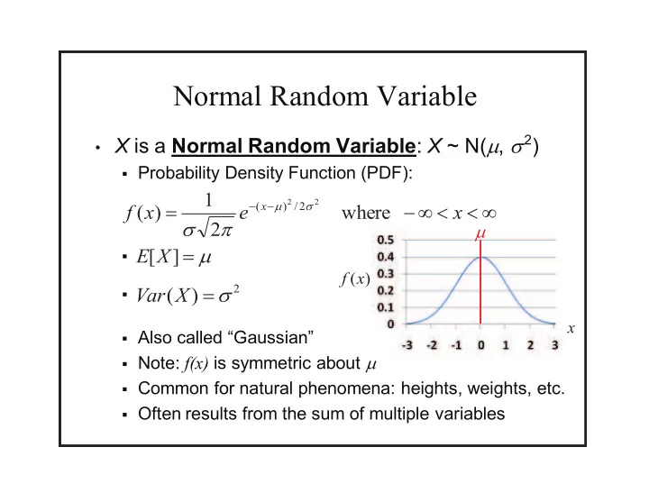
• X is a Normal Random Variable: X ~ N(, 2)

Probability Density Function (PDF):

• Also called “Gaussian”

Note: f(x) is symmetric about Common for natural phenomena: heights, weights, etc. Often results from the sum of multiple variables

• x

e x f

x

where 2 1 ) (

2 2 2

/ ) (

• ]

[X E

2

) (

• X

Var

) (x f x

Carl Friedrich Gauss

• Carl Friedrich Gauss (1777-1855) was a

remarkably influential German mathematician

• Started doing groundbreaking math as teenager

Did not invent Normal distribution, but popularized it

• He looked more like Martin Sheen

Who is, of course, Charlie Sheen’s father

Properties of Normal Random Variable

• Let X ~ N(, 2)
• Let Y = aX + b

Y ~ N(a + b, a2 2) E[Y] = E[aX + b] = aE[X] + b = a + b Var(Y) = Var(aX + b) = a2Var(X) = a2 2

Differentiating FY(x) w.r.t. x , yields fY(x), the PDF for y:

• Special case: Z = (X – )/

(a = 1/ , b = –/)

Z ~ N(a + b, a2 2) = N(/ – /, (1/22) = N(0, 1)

) ( ) ( ) ( ) ( ) (

a b x a b x

X Y

F X P x b aX P x Y P x F

• )

( ) ( ) ( ) (

1

a b x a a b x dx d dx d

X X Y Y

f F x F x f

Standard (Unit) Normal Random Variable

• Z is a Standard (or Unit) Normal RV: Z ~ N(0, 1)

E[Z] = = 0

Var(Z) = 2 = 1 SD(Z) = = 1

CDF of Z, FZ(z) does not have closed form We denote FZ(z) as (z): “phi of z” By symmetry: (–z) = P(Z ≤ –z) = P(Z ≥ z) = 1 – (z)

• Use Z to compute X ~ N(, 2), where > 0

Table of (z) values in textbook, p. 201 and handout

dx e dx e z Z P z

z x z x

• 2

/ 2 / ) (

2 2 2

2 1 2 1 ) ( ) Φ(

• )

( ) ( ) ( ) ( ) (

• x

x x X

Z P P x X P x FX

Using Table of (z) Values

(0.54) = 0.7054

• X ~ N(3, 16)

= 3 2 = 16 = 4

What is P(X > 0)? What is P(2 < X < 5)? What is P(|X – 3| > 6)?

Get Your Gaussian On

) 4 2 4 1 ) 4 3 5 4 3 4 3 2

( ( ) 5 2 (

• Z

P P X P

X

2902 . ) 5987 . 1 ( 6915 . )) ( 1 ( ) ( ) ( ) (

4 1 2 1 4 1 4 2

• 7734

. ) ( ) ( 1

4 3 4 3

• )

4 3 ) 4 3 4 3

( ( ) (

• Z

P P X P

X ) 4 3 9 ) 4 3 3

( ( ) 9 ( ) 3 (

• Z

P Z P X P X P 1336 . ) 9332 . 1 ( 2 )) ( 1 ( 2 )) ( 1 ( ) (

2 3 2 3 2 3

• Send voltage of 2 or -2 on wire (to denote 1 or 0)

X = voltage sent R = voltage received = X + Y, where noise Y ~ N(0, 1) Decode R: if (R ≥ 0.5) then 1, else 0 What is P(error after decoding | original bit = 1)? What is P(error after decoding | original bit = 0)?

Noisy Wires

0668 . ) 5 . 1 ( 1 ) 5 . 1 ( ) 5 . 1 ( ) 5 . 2 (

• Y

P Y P 0062 . ) 5 . 2 ( 1 ) 5 . 2 ( ) 5 . 2 (

• Y

P Y P

• X ~ Bin(n, p)

E[X] = np

Var(X) = np(1 – p)

Poisson approx. good: n large (> 20), p small (< 0.05) For large n: X Y ~ N(E[X], Var(X)) = N(np, np(1 – p)) Normal approx. good : Var(X) = np(1 – p) ≥ 10 DeMoivre-Laplace Limit Theorem:

• Sn: number of successes (with prob. p) in n independent trials

Normal Approximation to Binomial

• )

1 ( 5 . ) 1 ( 5 . ) (

2 1 2 1

p np np k p np np k k Y k P k X P ) ( ) ( ) 1 ( a b b p np np S a P

n n

Comparison when n = 100, p = 0.5

P(X = k) k )

• 100 people placed on special diet

X = # people on diet whose cholesterol decreases Doctor will endorse diet if X ≥ 65 What is P(doctor endorses diet | diet has no effect)? X ~ Bin(100, 0.5) Use Normal approximation: Y ~ N(50, 25) Using Binomial:

Faulty Endorsements

) 5 . 64 ( ) 65 (

• Y

P X P

• 0019

. ) 9 . 2 ( 1 ) 5 . 64 (

5 50 5 . 64 5 50

• Y

P Y P 0018 . ) 65 (

• X

P 5 1 25 1 50 – p) np( – p) np( np

• Stanford accepts 2480 students

Each accepted student has 68% chance of attending X = # students who will attend. X ~ Bin(2480, 0.68) What is P(X > 1745)? Use Normal approximation: Y ~ N(1686.4, 539.65) Using Binomial:

Stanford Admissions

) 5 . 1745 ( ) 1745 (

• Y

P X P 23 . 23 1 65 . 539 1 4 . 1686 – p) np( – p) np( np

• 0055

. ) 54 . 2 ( 1 ) 5 . 1745 (

23 . 23 4 . 1686 5 . 1745 23 . 23 4 . 1686

• Y

P Y P 0053 . ) 1745 (

• X

P

Exponential Random Variable

• X is an Exponential RV: X ~ Exp() Rate: > 0

Probability Density Function (PDF):

• Cumulative distribution function (CDF), F(X) = P(X x):

Represents time until some event

• Earthquake, request to web server, end cell phone contract, etc.
• x

where if if ) ( x x e x f

x

• 1

] [

• X

E

2

1 ) (

• X

Var

(CDF), (X) P( ):

) (x f x

where 1 ) (

• x

e x F

x

• X = time until some event occurs

X ~ Exp() What is P(X > s + t | X > s)? After initial period of time s, P(X > t | ) for waiting

another t units of time until event is same as at start

“Memoryless” = no impact from preceding period s

Exponential is “Memoryless”

) ( ) ( ) ( ) and ( ) | ( s X P t s X P s X P s X t s X P s X t s X P

• )

( ) ( 1 ) ( 1 ) ( 1 ) ( ) (

) (

t X P t F e e e s F t s F s X P t s X P

t s t s

• )

( ) | ( So, t X P s X t s X P

• Say a visitor to your web leaves after X minutes

On average, visitors leave site after 5 minutes Assume length of stay is Exponentially distributed X ~ Exp( = 1/5), since E[X] = 1/ = 5 What is P(X > 10)? What is P(10 < X < 20)?

Visits to Web Site

1353 . ) 1 ( 1 ) 10 ( 1 ) 10 (

2 10

• e

e F X P

• 1170

. ) 1 ( ) 1 ( ) 10 ( ) 20 ( ) 20 10 (

2 4

• e

e F F X P

• X = # hours of use until your laptop dies

On average, laptops die after 5000 hours of use X ~ Exp( = 1/5000), since E[X] = 1/ = 5000 You use your laptop 5 hours/day. What is P(your laptop lasts 4 years)? That is: P(X > (5)(365)(4) = 7300) Better plan ahead... especially if you are coterming:

Replacing Your Laptop

2322 . ) 1 ( 1 ) 7300 ( 1 ) 7300 (

46 . 1 5000 / 7300

• e

e F X P plan) year (5 1612 . ) 9125 ( 1 ) 9125 (

825 . 1

• e

F X P plan) year (6 1119 . ) 10950 ( 1 ) 10950 (

19 . 2

• e

F X P

• Product rule for derivatives:
• Derivative and integral of exponential:
• Integration by parts:

A Little Calculus Review

dv u v du v u d

• )

(

dx du e dx e d

u u

• )

(

• dv

u du v v u v u d ) (

• du

v v u dv u

u u

e du e

• Compute n-th moment of Exponential distribution

Step 1: don’t panic, think happy thoughts, recall... Step 2: find u and v (and du and dv): Step 3: substitute (a.k.a. “plug and chug”)

And Now, Some Calculus Practice

• ]

[ dx e x X E

x n n

• x

n

e v x u

• dx

e dv dx nx du

x n

• 1
• dx

e nx e x du v v u dx e x dv u

x n x n x n

• 1

] [ ] [

1 1 1

• n

x n x n x n n

X E dx e x dx e nx e x X E

n n

• ,...

] [ ] [ so , 1 ] 1 [ ] [ : case Base

2 2

2 1 2 , 1

• X

E X E E X E