28. How to compute the flux Lets start with the case when S is the - - PDF document

• 28. How to compute the flux

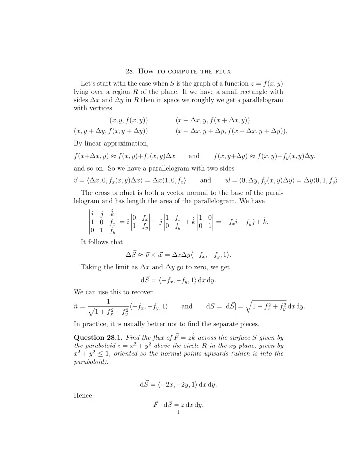
Let’s start with the case when S is the graph of a function z = f(x, y) lying over a region R of the plane. If we have a small rectangle with sides ∆x and ∆y in R then in space we roughly we get a parallelogram with vertices (x, y, f(x, y)) (x + ∆x, y, f(x + ∆x, y)) (x, y + ∆y, f(x, y + ∆y)) (x + ∆x, y + ∆y, f(x + ∆x, y + ∆y)). By linear approximation, f(x+∆x, y) ≈ f(x, y)+fx(x, y)∆x and f(x, y+∆y) ≈ f(x, y)+fy(x, y)∆y. and so on. So we have a parallelogram with two sides

• v = ∆x, 0, fx(x, y)∆x = ∆x1, 0, fx

and

• w = 0, ∆y, fy(x, y)∆y = ∆y0, 1, fy.

The cross product is both a vector normal to the base of the paral- lelogram and has length the area of the parallelogram. We have

• ˆ

ı ˆ  ˆ k 1 fx 1 fy

• = ˆ

ı

• fx

1 fy

• − ˆ



• 1

fx fy

• + ˆ

k

• 1

1

• = −fxˆ

ı − fyˆ  + ˆ k. It follows that ∆ S ≈ v × w = ∆x∆y−fx, −fy, 1. Taking the limit as ∆x and ∆y go to zero, we get d S = −fx, −fy, 1 dx dy. We can use this to recover ˆ n = 1 1 + f 2

x + f 2 y

−fx, −fy, 1 and dS = |d S| =

• 1 + f 2

x + f 2 y dx dy.

In practice, it is usually better not to find the separate pieces. Question 28.1. Find the flux of F = zˆ k across the surface S given by the paraboloid z = x2 + y2 above the circle R in the xy-plane, given by x2 + y2 ≤ 1, oriented so the normal points upwards (which is into the paraboloid). d S = −2x, −2y, 1 dx dy. Hence

• F · d

S = z dx dy.

1

So the flux is

• S
• F · d

S =

• R

z dx dy = 2π 1 r3 dr dθ. The inner integral is 1 r3 dr = r4 4 1 = 1 4. The outer integral is 2π 1 4 dθ = π 2 . More generally, suppose S is given as a parametric surface x(u, v), y(u, v) and z(u, v), then we can integrate using u and v, so that r =

• r(u, v). Arguing as above,

d S = ∂ r ∂u × ∂ r ∂v du dv. Apart from parametrisations, a surface S might be given by a con-

• straint. S might be given implicitly, by an equation g(x, y, z) = 0. In

this case

• N = ∇g = gx, gy, gz,

is normal to S and so ˆ n =

• N

| N| is a unit normal. To get ∆S, consider the projection to the xy-plane (assume that the plane is not vertical; if it is vertical, just project onto the xz-plane or the yz-plane). The key point is to figure out how area changes under

• projection. I claim

∆A = cos α∆S, where α is the angle of the surface with the horizontal, that is, the angle between N and the vertical ˆ

• k. The reason for this is the same

reason that the projection of a circle, lying in a slanted plane, is an

• ellipse. Note that every plane contains one horizontal line. To figure
• ut how area changes under projection, one can rotate the plane so that

this line is the y-axis. So lengths in the y direction are unchanged. In the x-direction, one gets a right angled triangle. The original length is a hypotenuse and the new length is the adjacent. So lengths in the x-direction scale by cos α. In total the area scales by cos α. But

• N · ˆ

k = |N| cos α.

2

Putting all of this together, d S =

• N

| N.ˆ k| dx dy. Example 28.2. Suppose that g(x, y, z) = z − f(x, y), so that g = 0 defines the graph of f. Then

• N = ∇g = −fx, −fy, 1

and

• N · ˆ

k = 1, so we get the old formula. Theorem 28.3 (Divergence Theorem). Let S be a closed surface bound- ing a solid D, oriented outwards. Let F be a vector field with continuous partial derivatives. Then

• S
• F · d

S =

• D

div F dV where div F = Px + Qy + Rz. This has the same physical interpretation as before. The total amount

• f material leaving S is equal to the amount of material created (or de-

stroyed) inside the solid D. Example 28.4. Let F = zˆ k and let S be the surface of a sphere of radius a. div F = 0 + 0 + 1 = 1, and so

• S
• F · d

S =

• D

div F dV =

• D

1 dV = 4 3πa3. It is convenient to introduce some symbolic notation. ∇ = ∂ ∂x, ∂ ∂y, ∂ ∂z is called the del operator. ∇f = ∂f ∂x, ∂f ∂y , ∂f ∂z is the gradient. We have div F = ∇ · F = ∂ ∂x, ∂ ∂y, ∂ ∂z · P, Q, R = ∂P ∂x + ∂Q ∂y + ∂R ∂z . is the divergence.

3