14. Stochastic Processes Introduction Let denote the random - - PowerPoint PPT Presentation

1

• 14. Stochastic Processes

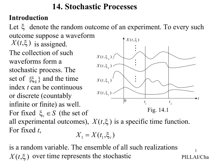
Let denote the random outcome of an experiment. To every such

• utcome suppose a waveform

is assigned. The collection of such waveforms form a stochastic process. The set of and the time index t can be continuous

• r discrete (countably

infinite or finite) as well. For fixed (the set of all experimental outcomes), is a specific time function. For fixed t, is a random variable. The ensemble of all such realizations

• ver time represents the stochastic

ξ ) , ( ξ t X } { k ξ S

i ∈

ξ ) , ( 1

1 i

t X X ξ = ) , ( ξ t X

PILLAI/Cha

t

1

t

2

t ) , (

n

t X ξ ) , (

k

t X ξ ) , (

2

ξ t X ) , (

1

ξ t X

• Fig. 14.1

) , ( ξ t X

) , ( ξ t X Introduction

2

process X(t). (see Fig 14.1). For example where is a uniformly distributed random variable in represents a stochastic process. Stochastic processes are everywhere: Brownian motion, stock market fluctuations, various queuing systems all represent stochastic phenomena. If X(t) is a stochastic process, then for fixed t, X(t) represents a random variable. Its distribution function is given by Notice that depends on t, since for a different t, we obtain a different random variable. Further represents the first-order probability density function of the process X(t). ), cos( ) ( ϕ ω + = t a t X ϕ } ) ( { ) , ( x t X P t x FX ≤ = ) , ( t x FX (14-1) (14-2)

PILLAI/Cha

(0,2 ), π dx t x dF t x f

X X

) , ( ) , ( =

∆

3

For t = t1 and t = t2, X(t) represents two different random variables X1 = X(t1) and X2 = X(t2) respectively. Their joint distribution is given by and represents the second-order density function of the process X(t). Similarly represents the nth order density function of the process X(t). Complete specification of the stochastic process X(t) requires the knowledge of for all and for all n. (an almost impossible task in reality). } ) ( , ) ( { ) , , , (

2 2 1 1 2 1 2 1

x t X x t X P t t x x FX ≤ ≤ = (14-3) (14-4) ) , , , , , (

2 1 2 1 n n

t t t x x x f X

• )

, , , , , (

2 1 2 1 n n

t t t x x x f X

• n

i ti , , 2 , 1 ,

• =

PILLAI/Cha

2 1 2 1 2 1 2 1 2 1 2

( , , , ) ( , , , )

X X

F x x t t f x x t t x x ∂ = ∂ ∂

∆

4

Mean of a Stochastic Process: represents the mean value of a process X(t). In general, the mean of a process can depend on the time index t. Autocorrelation function of a process X(t) is defined as and it represents the interrelationship between the random variables X1 = X(t1) and X2 = X(t2) generated from the process X(t). Properties: 1. 2. (14-5) (14-6)

* 1 * 2 1 2 * 2 1

)}] ( ) ( { [ ) , ( ) , ( t X t X E t t R t t R

XX XX

= = (14-7) . } | ) ( {| ) , (

2 >

= t X E t t RXX

PILLAI/Cha

(Average instantaneous power) ( ) { ( )} ( , )

X

t E X t x f x t dx µ

+∞ −∞

= = ∫

∆ * * 1 2 1 2 1 2 1 2 1 2 1 2

( , ) { ( ) ( )} ( , , , )

XX X

R t t E X t X t x x f x x t t dx dx = = ∫∫

∆

5

• 3. represents a nonnegative definite function, i.e., for any

set of constants

• Eq. (14-8) follows by noticing that

The function represents the autocovariance function of the process X(t). Example 14.1 Let Then . ) ( for } | {|

1 2

∑

=

= ≥

n i i i

t X a Y Y E ) ( ) ( ) , ( ) , (

2 * 1 2 1 2 1

t t t t R t t C

X X XX XX

µ µ − = (14-9) . ) (

∫−

=

T T

dt t X z

∫ ∫ ∫ ∫

− − − −

= =

T T T T T T T T

dt dt t t R dt dt t X t X E z E

XX

2 1 2 1 2 1 2 * 1 2

) , ( )} ( ) ( { ] | [| (14-10)

n i i

a

1

} {

=

) , (

2 1 t

t RXX

∑∑

= =

≥

n i n j j i j i

t t R a a

XX

1 1 *

. ) , ( (14-8)

PILLAI/Cha

6

Similarly , } {sin sin } {cos cos )} {cos( )} ( { ) ( = − = + = = ϕ ω ϕ ω ϕ ω µ E t a E t a t aE t X E t

X

). ( cos 2 )} 2 ) ( cos( ) ( {cos 2 )} cos( ) {cos( ) , (

2 1 2 2 1 2 1 2 2 1 2 2 1

t t a t t t t E a t t E a t t RXX − = + + + − = + + = ω ϕ ω ω ϕ ω ϕ ω (14-12) (14-13) Example 14.2 ). 2 , ( ~ ), cos( ) ( π ϕ ϕ ω U t a t X + = (14-11) This gives

PILLAI/Cha

∫

= = =

π

ϕ ϕ ϕ ϕ

π

2

}. {sin cos } {cos since

2 1

E d E

7

Stationary Stochastic Processes

Stationary processes exhibit statistical properties that are invariant to shift in the time index. Thus, for example, second-order stationarity implies that the statistical properties of the pairs {X(t1) , X(t2) } and {X(t1+c) , X(t2+c)} are the same for any c. Similarly first-order stationarity implies that the statistical properties

• f X(ti) and X(ti+c) are the same for any c.

In strict terms, the statistical properties are governed by the joint probability density function. Hence a process is nth-order Strict-Sense Stationary (S.S.S) if for any c, where the left side represents the joint density function of the random variables and the right side corresponds to the joint density function of the random variables A process X(t) is said to be strict-sense stationary if (14-14) is true for all ) , , , , , ( ) , , , , , (

2 1 2 1 2 1 2 1

c t c t c t x x x f t t t x x x f

n n n n

X X

+ + + ≡

• (14-14)

) ( , ), ( ), (

2 2 1 1 n n

t X X t X X t X X = = =

• ).

( , ), ( ), (

2 2 1 1

c t X X c t X X c t X X

n n

+ = ′ + = ′ + = ′

• .

and , 2 , 1 , , , 2 , 1 , c any n n i ti

• =

=

PILLAI/Cha

8

For a first-order strict sense stationary process, from (14-14) we have for any c. In particular c = – t gives i.e., the first-order density of X(t) is independent of t. In that case Similarly, for a second-order strict-sense stationary process we have from (14-14) for any c. For c = – t2 we get ) , ( ) , ( c t x f t x f

X X

+ ≡ (14-16) (14-15) (14-17) ) ( ) , ( x f t x f

X X

= [ ( )] ( ) , E X t x f x dx a constant. µ

+∞ −∞

= =

∫

) , , , ( ) , , , (

2 1 2 1 2 1 2 1

c t c t x x f t t x x f

X X

+ + ≡ ) , , ( ) , , , (

2 1 2 1 2 1 2 1

t t x x f t t x x f

X X

− ≡ (14-18)

PILLAI/Cha

9

i.e., the second order density function of a strict sense stationary process depends only on the difference of the time indices In that case the autocorrelation function is given by i.e., the autocorrelation function of a second order strict-sense stationary process depends only on the difference of the time indices Notice that (14-17) and (14-19) are consequences of the stochastic process being first and second-order strict sense stationary. On the other hand, the basic conditions for the first and second order stationarity – Eqs. (14-16) and (14-18) – are usually difficult to verify. In that case, we often resort to a looser definition of stationarity, known as Wide-Sense Stationarity (W.S.S), by making use of .

2 1

τ = − t t .

2 1

t t − = τ (14-19)

PILLAI/Cha

* 1 2 1 2 * 1 2 1 2 1 2 1 2 * 1 2

( , ) { ( ) ( )} ( , , ) ( ) ( ) ( ),

XX X XX XX XX

R t t E X t X t x x f x x t t dx dx R t t R R τ τ τ = = = − = − = = −

∫∫

∆ ∆

10

(14-17) and (14-19) as the necessary conditions. Thus, a process X(t) is said to be Wide-Sense Stationary if (i) and (ii) i.e., for wide-sense stationary processes, the mean is a constant and the autocorrelation function depends only on the difference between the time indices. Notice that (14-20)-(14-21) does not say anything about the nature of the probability density functions, and instead deal with the average behavior of the process. Since (14-20)-(14-21) follow from (14-16) and (14-18), strict-sense stationarity always implies wide-sense stationarity. However, the converse is not true in general, the only exception being the Gaussian process. This follows, since if X(t) is a Gaussian process, then by definition are jointly Gaussian random variables for any whose joint characteristic function is given by µ = )} ( { t X E (14-21) (14-20) ), ( )} ( ) ( {

2 1 2 * 1

t t R t X t X E

XX

− = ) ( , ), ( ), (

2 2 1 1 n n

t X X t X X t X X = = =

• PILLAI/Cha

n

t t t , , 2

1

11

where is as defined on (14-9). If X(t) is wide-sense stationary, then using (14-20)-(14-21) in (14-22) we get and hence if the set of time indices are shifted by a constant c to generate a new set of jointly Gaussian random variables then their joint characteristic function is identical to (14-23). Thus the set of random variables and have the same joint probability distribution for all n and all c, establishing the strict sense stationarity of Gaussian processes from its wide-sense stationarity. To summarize if X(t) is a Gaussian process, then wide-sense stationarity (w.s.s) strict-sense stationarity (s.s.s). Notice that since the joint p.d.f of Gaussian random variables depends

• nly on their second order statistics, which is also the basis

) , (

k i t

t CXX

1 ,

( ) ( , ) / 2 1 2

( , , , )

XX

n n k k i k i k k l k X

j t C t t n

e

µ ω ω ω

φ ω ω ω

=

−

∑ ∑∑ =

• (14-22)

1 2 1 1 1 1

( ) 1 2

( , , , )

XX

n n n k i k i k k k X

j C t t n

e

µω ω ω

φ ω ω ω

= = =

− −

∑ ∑∑ =

• (14-23)

n i i

X

1

} {

= n i i

X

1

} {

=

′ ⇒

PILLAI/Cha

), ( 1

1

c t X X + = ′ ) ( , ), (

2 2

c t X X c t X X

n n

+ = ′ + = ′

12

for wide sense stationarity, we obtain strict sense stationarity as well. From (14-12)-(14-13), (refer to Example 14.2), the process in (14-11) is wide-sense stationary, but not strict-sense stationary. Similarly if X(t) is a zero mean wide sense stationary process in Example 14.1, then in (14-10) reduces to As t1, t2 varies from –T to +T, varies from –2T to + 2T. Moreover is a constant

• ver the shaded region in Fig 14.2, whose area is given by

and hence the above integral reduces to ), cos( ) ( ϕ ω + = t a t X

PILLAI/Cha

2 z

σ . ) ( } | {|

2 1 2 1 2 2

∫ ∫

− −

− = =

T T T T z

dt dt t t R z E

XX

σ

2 1

t t − = τ ) (τ

XX

R ) ( > τ τ τ τ τ τ d T d T T ) 2 ( ) 2 ( 2 1 ) 2 ( 2 1

2 2

− = − − − − . ) 1 )( ( |) | 2 )( (

2 2 2 | | 2 1 2 2 2

∫ ∫

− −

− = − =

T t T T T t z

d R d T R

XX XX

τ τ τ τ τ σ

τ

(14-24)

T −

T T − τ τ τ − T 2

2

t

1

t

• Fig. 14.2

2 1

t t − = τ

13

Systems with Stochastic Inputs

A deterministic system1 transforms each input waveform into an output waveform by operating only on the time variable t. Thus a set of realizations at the input corresponding to a process X(t) generates a new set of realizations at the

• utput associated with a new process Y(t).

) , (

i

t X ξ )] , ( [ ) , (

i i

t X T t Y ξ ξ = )} , ( { ξ t Y Our goal is to study the output process statistics in terms of the input process statistics and the system function.

1A stochastic system on the other hand operates on both the variables t and

. ξ PILLAI/Cha

] [⋅ T   → 

) (t X

 → 

) (t Y t t ) , (

i

t X ξ ) , (

i

t Y ξ

• Fig. 14.3

14

Deterministic Systems

Systems with Memory Time-Invariant systems Linear systems Linear-Time Invariant (LTI) systems Memoryless Systems )] ( [ ) ( t X g t Y = )] ( [ ) ( t X L t Y =

PILLAI/Cha

Time-varying systems

• Fig. 14.3

. ) ( ) ( ) ( ) ( ) (

∫ ∫

∞ + ∞ − ∞ + ∞ −

− = − = τ τ τ τ τ τ d t X h d X t h t Y ( ) h t ( ) X t LTI system

15

Memoryless Systems:

The output Y(t) in this case depends only on the present value of the input X(t). i.e., (14-25)

PILLAI/Cha

)} ( { ) ( t X g t Y = Memoryless system Memoryless system Memoryless system Strict-sense stationary input Wide-sense stationary input X(t) stationary Gaussian with ) (τ

XX

R Strict-sense stationary output. Need not be stationary in any sense. Y(t) stationary,but not Gaussian with (see (14-26)). ). ( ) ( τ η τ

XX XY

R R = (see (9-76), Text for a proof.)

• Fig. 14.4

16

Theorem: If X(t) is a zero mean stationary Gaussian process, and Y(t) = g[X(t)], where represents a nonlinear memoryless device, then Proof: where are jointly Gaussian random variables, and hence ) (⋅ g )}. ( { ), ( ) ( X g E R R

XX XY

′ = = η τ η τ (14-26)

2 1 2 1 2 1

) , ( ) ( )}] ( { ) ( [ )} ( ) ( { ) (

2 1

dx dx x x f x g x t X g t X E t Y t X E R

X X XY

∫∫

= − = − = τ τ τ (14-27) ) ( ), (

2 1

τ − = = t X X t X X

PILLAI/Cha

* 1 1 2

/ 2 1 2 1 2 1 2 * *

1 2 | | (0) ( ) ( ) (0)

( , ) ( , ) , ( , ) { }

XX XX XX XX

X X

x A x T T

A R R R R

f x x e X X X x x x A E X X LL

π τ τ

−

−

= = =   = = =    

∆

17

where L is an upper triangular factor matrix with positive diagonal

• entries. i.e.,

Consider the transformation so that and hence Z1, Z2 are zero mean independent Gaussian random

• variables. Also

and hence The Jacobaian of the transformation is given by .

22 12 11

      = l l l L I AL L L X X E L Z Z E = = =

− −

− −

1 1

* 1 * * 1 *

} { } {

* * * 1 * 1 2 2 1 2.

x A x z L A Lz z z z z

− −

= = = +

2 22 2 2 12 1 11 1

, z l x z l z l x z L x = + = ⇒ =

PILLAI/Cha

1 1 1 2 1 2

( , ) , ( , )

T T

Z L X Z Z z L x z z

− −

= = = =

∆ ∆

18

Hence substituting these into (14-27), we obtain where This gives . | | | | | |

2 / 1 1 − − =

= A L J

2 2 1 2 1/2 11 1 12 2 22 2 11 1 22 2 1 2 1 2 12 2 22 2 1 2 1 2

/ 2 / 2 1 1 | | 2 | | 1 2 1 2

( ) ( ) ( ) ( ) ( ) ( ) ( ) ( ) ( )

XY

J A z z z z

z z

R l z l z g l z e e l z g l z f z f z dz dz l z g l z f z f z dz dz

π

τ

+∞ +∞ − − −∞ −∞ +∞ +∞ −∞ −∞ +∞ +∞ −∞ −∞

= + ⋅ = + =

∫ ∫ ∫ ∫ ∫ ∫

2 2 2 12 22 22

11 1 1 22 2 2 1 2 12 2 22 2 2 2 /2 2 2

1 2 2 1 2 / 2 1 2

( ) ( ) ( ) ( ) ( ) ( ) ,

z z z z u

l

l l

l z f z dz g l z f z dz l z g l z f z dz e ug u e du

π π

−

+∞ +∞ −∞ −∞ +∞ −∞ +∞ − −∞

+ =

∫ ∫ ∫ ∫

• PILLAI/Cha

22 2.

u l z =

19

2 22 2 22 22

2 2

( ) / 2 1 12 22 2 ( ) ( )

( ) ( ) ( ) ( ) ( ) ,

u XY u u XX

f u u df u f u du u

l l

u l

R l l g u e du R g u f u du

π

τ τ

+∞ − −∞ ′ − =− +∞ −∞

= ′ = −

∫ ∫

• Hence

). ( gives since

22 12 *

τ

XX

R l l LL A = = the desired result, where Thus if the input to a memoryless device is stationary Gaussian, the cross correlation function between the input and the output is proportional to the input autocorrelation function.

PILLAI/Cha

), ( )} ( { ) ( } ) ( ) ( | ) ( ) ( ){ ( ) ( τ η τ τ τ

XX XX XX XY

R X g E R du u f u g u f u g R R

u u

= ′ = ′ + − =

∫

∞ + ∞ − ∞ + ∞ −

)]. ( [ X g E ′ = η

20

Linear Systems:

represents a linear system if Let represent the output of a linear system. Time-Invariant System: represents a time-invariant system if i.e., shift in the input results in the same shift in the output also. If satisfies both (14-28) and (14-30), then it corresponds to a linear time-invariant (LTI) system. LTI systems can be uniquely represented in terms of their output to a delta function ] [⋅ L )} ( { ) ( t X L t Y = )}. ( { )} ( { )} ( ) ( {

2 2 1 1 2 2 1 1

t X L a t X L a t X a t X a L + = + (14-28) ] [⋅ L ) ( )} ( { )} ( { ) ( t t Y t t X L t X L t Y − = − ⇒ = (14-29) (14-30) ] [⋅ L

PILLAI/Cha

LTI ) (t δ ) (t h

Impulse Impulse response of the system

t ) (t h

Impulse response

• Fig. 14.5

21

• Eq. (14-31) follows by expressing X(t) as

and applying (14-28) and (14-30) to Thus )}. ( { ) ( t X L t Y =

∫

∞ + ∞ −

− = ) ( ) ( ) ( τ τ δ τ d t X t X (14-31) (14-32) (14-33)

PILLAI/Cha

. ) ( ) ( ) ( ) ( )} ( { ) ( } ) ( ) ( { } ) ( ) ( { )} ( { ) (

∫ ∫ ∫ ∫ ∫

∞ + ∞ − ∞ + ∞ − ∞ + ∞ − ∞ + ∞ − ∞ + ∞ −

− = − = − = − = − = = τ τ τ τ τ τ τ τ δ τ τ τ δ τ τ τ δ τ d t X h d t h X d t L X d t X L d t X L t X L t Y

By Linearity By Time-invariance

then LTI

∫ ∫

∞ + ∞ − ∞ + ∞ −

− = − = ) ( ) ( ) ( ) ( ) ( τ τ τ τ τ τ d t X h d X t h t Y

arbitrary input

t ) (t X t ) (t Y

• Fig. 14.6

) (t X ) (t Y

22

Output Statistics: Using (14-33), the mean of the output process

is given by Similarly the cross-correlation function between the input and output processes is given by Finally the output autocorrelation function is given by ). ( ) ( ) ( ) ( } ) ( ) ( { )} ( { ) ( t h t d t h d t h X E t Y E t

X X Y

∗ = − = − = =

∫ ∫

∞ + ∞ − ∞ + ∞ −

µ τ τ τ µ τ τ τ µ (14-34) ). ( ) , ( ) ( ) , ( ) ( )} ( ) ( { } ) ( ) ( ) ( { )} ( ) ( { ) , (

2 * 2 1 * 2 1 * 2 1 * 2 1 2 * 1 2 1

t h t t R d h t t R d h t X t X E d h t X t X E t Y t X E t t R

XX XX XY

∗ = − = − = − = =

∫ ∫ ∫

∞ + ∞ − ∞ + ∞ − ∞ + ∞ −

α α α α α α α α α

* *

(14-35)

PILLAI/Cha

23

• r

), ( ) , ( ) ( ) , ( ) ( )} ( ) ( { } ) ( ) ( ) ( { )} ( ) ( { ) , (

1 2 1 2 1 2 1 2 * 1 2 * 1 2 1

t h t t R d h t t R d h t Y t X E t Y d h t X E t Y t Y E t t R

XY XY YY

∗ = − = − = − = =

∫ ∫ ∫

∞ + ∞ − ∞ + ∞ − ∞ + ∞ −

β β β β β β β β β

*

). ( ) ( ) , ( ) , (

1 2 * 2 1 2 1

t h t h t t R t t R

XX YY

∗ ∗ = (14-36) (14-37)

PILLAI/Cha

h(t) ) (t

X

µ ) (t

Y

µ h*(t2) h(t1)    → 

) , (

2 1 t

t RXY

→  →  ) , (

2 1 t

t RYY ) , (

2 1 t

t RXX

(a) (b)

• Fig. 14.7

24

In particular if X(t) is wide-sense stationary, then we have so that from (14-34) Also so that (14-35) reduces to Thus X(t) and Y(t) are jointly w.s.s. Further, from (14-36), the output autocorrelation simplifies to From (14-37), we obtain

X X t

µ µ = ) ( constant. a c d h t

X X Y

, ) ( ) ( µ τ τ µ µ = =

∫

∞ + ∞ −

(14-38) ) ( ) , (

2 1 2 1

t t R t t R

XX XX

− = (14-39) ). ( ) ( ) ( , ) ( ) ( ) , (

2 1 2 1 2 1

τ τ τ τ β β β

YY XY XY YY

R h R t t d h t t R t t R = ∗ = − = − − = ∫

∞ + ∞ −

(14-40) ). ( ) ( ) ( ) (

*

τ τ τ τ h h R R

XX YY

∗ − ∗ = (14-41)

PILLAI/Cha

. ), ( ) ( ) ( ) ( ) ( ) , (

2 1 * * 2 1 2 1

t t R h R d h t t R t t R

XY XX XX XY

− = = − ∗ = + − = ∫

∞ + ∞ −

τ τ τ τ α α α

∆

25

From (14-38)-(14-40), the output process is also wide-sense stationary. This gives rise to the following representation

PILLAI/Cha

LTI system h(t) Linear system wide-sense stationary process strict-sense stationary process Gaussian process (also stationary) wide-sense stationary process. strict-sense stationary process (see Text for proof ) Gaussian process (also stationary) ) (t X ) (t Y LTI system h(t) ) (t X ) (t X ) (t Y ) (t Y (a) (b) (c)

• Fig. 14.8

26

White Noise Process:

W(t) is said to be a white noise process if i.e., E[W(t1) W*(t2)] = 0 unless t1 = t2. W(t) is said to be wide-sense stationary (w.s.s) white noise if E[W(t)] = constant, and If W(t) is also a Gaussian process (white Gaussian process), then all of its samples are independent random variables (why?). For w.s.s. white noise input W(t), we have ), ( ) ( ) , (

2 1 1 2 1

t t t q t t RWW − = δ (14-42) ). ( ) ( ) , (

2 1 2 1

τ δ δ q t t q t t RWW = − = (14-43) White noise W(t) LTI h(t) Colored noise ( ) ( ) ( ) N t h t W t = ∗

PILLAI/Cha

• Fig. 14.9

27

and where Thus the output of a white noise process through an LTI system represents a (colored) noise process. Note: White noise need not be Gaussian. “White” and “Gaussian” are two different concepts! ) ( ) ( ) ( ) ( ) ( ) ( ) (

* *

τ ρ τ τ τ τ τ δ τ q h qh h h q Rnn = ∗ − = ∗ − ∗ = (14-45) . ) ( ) ( ) ( ) ( ) (

* *

∫

∞ + ∞ −

+ = − ∗ = α τ α α τ τ τ ρ d h h h h (14-46)

PILLAI/Cha

(14-44) [ ( )] ( ) ,

W

E N t h d µ τ τ

+∞ −∞

=

∫

a constant

28

Upcrossings and Downcrossings of a stationary Gaussian process: Consider a zero mean stationary Gaussian process X(t) with autocorrelation function An upcrossing over the mean value

• ccurs whenever the realization X(t)

passes through zero with positive slope. Let represent the probability

• f such an upcrossing in

the interval We wish to determine Since X(t) is a stationary Gaussian process, its derivative process is also zero mean stationary Gaussian with autocorrelation function (see (9-101)-(9-106), Text). Further X(t) and are jointly Gaussian stationary processes, and since (see (9-106), Text) ). (τ

XX

R t ∆ ρ ). , ( t t t ∆ + . ρ

• Fig. 14.10

) (t X ′ ) ( ) ( τ τ

XX X X

R R ′ ′ − =

′ ′

) (t X ′ , ) ( ) ( τ τ τ d dR R

XX X X

− =

′

PILLAI/Cha Upcrossings

t ) (t X

Downcrossing

29

we have which for gives i.e., the jointly Gaussian zero mean random variables are uncorrelated and hence independent with variances

• respectively. Thus

To determine the probability of upcrossing rate, = τ ) ( ) ( ) ( ) ( ) ( τ τ τ τ τ τ

X X XX XX X X

R d dR d dR R

′ ′

− = = − − − = − (14-48) (14-47) (0) [ ( ) ( )]

XX

R E X t X t

′

′ = ⇒ = ) ( and ) (

2 1

t X X t X X ′ = = (14-49) , ρ ) ( ) ( and ) (

2 2 2 1

> ′ ′ − = = =

′ ′ XX X X XX

R R R σ σ (14-50)

2 2 1 1 2 2 1 2 1 2

1 2 1 2 1 2

2 2

1 ( , ) ( ) ( ) . 2

X X X X

x x

f x x f x f x e

σ σ

πσ σ

  −   

+

= = (14-51)

PILLAI/Cha

30

PILLAI/Cha

we argue as follows: In an interval the realization moves from X(t) = X1 to and hence the realization intersects with the zero level somewhere in that interval if i.e., Hence the probability of upcrossing in is given by Differentiating both sides of (14-53) with respect to we get and letting Eq. (14-54) reduce to ), , ( t t t ∆ + , ) ( ) ( ) (

2 1

t X X t t X t X t t X ∆ + = ∆ ′ + = ∆ +

1 2

. X X t > − ∆ (14-52) ) , ( t t t ∆ + (14-53)

t ) (t X ) (t X ) ( t t X ∆ + t t t ∆ +

• Fig. 14.11

. ) ( ) ( ) , (

1 1 2 2 2 1 2 1

2 1 2 2 2 1 2 1

x d x f x d x f dx x d x x f t

t x x t x x

X X X X

∫ ∫ ∫ ∫

∞ ∆ − ∞ ∞ = ∆ − =

= = ∆ ρ , t ∆ (14-54)

2 1

2 2 2 2

( ) ( )

X X

f x x f x t dx ρ

∞

= − ∆

∫

, → ∆t

1 2 1 2

0, 0, and ( ) X X X t t X X t < > + ∆ = + ∆ >

31

PILLAI/Cha

[where we have made use of (5-78), Text]. There is an equal probability for downcrossings, and hence the total probability for crossing the zero line in an interval equals where It follows that in a long interval T, there will be approximately crossings of the mean value. If is large, then the autocorrelation function decays more rapidly as moves away from zero, implying a large random variation around the origin (mean value) for X(t), and the likelihood of zero crossings should increase with increase in agreeing with (14-56). ) ( ) ( 2 1 ) / 2 ( 2 1 ) ( 2 1 ) ( ) ( 2 1 ) ( ) (

2 2 2 2 2 2 2

XX XX XX X XX X X

R R R dx x f x R dx f x f x ′ ′ − = = = =

∫ ∫

∞ ∞

π π σ π π ρ (14-55) ) , ( t t t ∆ + ,

0 t

∆ ρ . ) ( / ) ( 1 > ′ ′ − =

XX XX

R R π ρ (14-56) T ρ ) (

XX

R ′ ′ − τ ) (τ

XX

R (0),

XX

R′′ −

32

Discrete Time Stochastic Processes: A discrete time stochastic process Xn = X(nT) is a sequence of random variables. The mean, autocorrelation and auto-covariance functions of a discrete-time process are gives by and

• respectively. As before strict sense stationarity and wide-sense

stationarity definitions apply here also. For example, X(nT) is wide sense stationary if and )} ( ) ( { ) , ( )} ( {

2 * 1 2 1

T n X T n X E n n R nT X E

n

= = µ

* 2 1 2 1

2 1

) , ( ) , (

n n

n n R n n C µ µ − = (14-57) (14-58) (14-59) constant a nT X E , )} ( { µ = (14-60)

PILLAI/Cha

(14-61)

* *

[ {( ) } {( ) }] ( )

n n

E X k n T X k T R n r r

−

+ = = =

∆

33

i.e., R(n1, n2) = R(n1 – n2) = R*(n2 – n1). The positive-definite property of the autocorrelation sequence in (14-8) can be expressed in terms of certain Hermitian-Toeplitz matrices as follows: Theorem: A sequence forms an autocorrelation sequence of a wide sense stationary stochastic process if and only if every Hermitian-Toeplitz matrix Tn given by is non-negative (positive) definite for Proof: Let represent an arbitrary constant vector. Then from (14-62), since the Toeplitz character gives Using (14-61),

• Eq. (14-63) reduces to

∞ + ∞ −

} { n r 0, 1, 2, , . n = ∞

• *

* 1 * 1 * 1 1 * 1 2 1 n n n n n n

T r r r r r r r r r r r r T =               =

− −

• T

n

a a a a ] , , , [

1

• =

(14-62)

PILLAI/Cha

∑∑

= = −

=

n i n k i k k i n

r a a a T a

* *

(14-63) . ) (

, i k k i n

r T

−

=

34

From (14-64), if X(nT) is a wide sense stationary stochastic process then Tn is a non-negative definite matrix for every Similarly the converse also follows from (14-64). (see section 9.4, Text) If X(nT) represents a wide-sense stationary input to a discrete-time system {h(nT)}, and Y(nT) the system output, then as before the cross correlation function satisfies and the output autocorrelation function is given by

• r

Thus wide-sense stationarity from input to output is preserved for discrete-time systems also. . , , 2 , 1 , ∞ =

• n

(14-64)

2 * * * *

{ ( ) ( )} ( ) 0.

n n n n i k k i k k

a T a a a E X kT X iT E a X kT

= = =

    = = ≥      

∑∑ ∑

PILLAI/Cha

) ( ) ( ) (

*

n h n R n R

XX XY

− ∗ = ) ( ) ( ) ( n h n R n R

XY YY

∗ = ). ( ) ( ) ( ) (

*

n h n h n R n R

XX YY

∗ − ∗ = (14-65) (14-66) (14-67)

35

Auto Regressive Moving Average (ARMA) Processes

Consider an input – output representation where X(n) may be considered as the output of a system {h(n)} driven by the input W(n). Z – transform of (14-68) gives

• r

, ) ( ) ( ) (

1

∑ ∑

= =

− + − − =

q k k p k k

k n W b k n X a n X (14-68) (14-69) h(n) W(n) X(n) ( ) ( ) , 1

p q k k k k k k

X z a z W z b z a

− − = =

= ≡

∑ ∑

∆

1 2 1 2 1 2 1 2

( ) ( ) ( ) ( ) ( ) ( ) 1

q q k p k p

b b z b z b z X z B z H z h k z W z A z a z a z a z

− − − ∞ − − − − =

+ + + + = = = = + + + +

∑

• (14-70)

PILLAI/Cha

Fig.14.12

36

represents the transfer function of the associated system response {h(n)} in Fig 14.12 so that Notice that the transfer function H(z) in (14-70) is rational with p poles and q zeros that determine the model order of the underlying system. From (14-68), the output undergoes regression over p of its previous values and at the same time a moving average based on

• f the input over (q + 1) values is added to it, thus

generating an Auto Regressive Moving Average (ARMA (p, q)) process X(n). Generally the input {W(n)} represents a sequence of uncorrelated random variables of zero mean and constant variance so that If in addition, {W(n)} is normally distributed then the output {X(n)} also represents a strict-sense stationary normal process. If q = 0, then (14-68) represents an AR(p) process (all-pole process), and if p = 0, then (14-68) represents an MA(q)

PILLAI/Cha

(14-72) (14-71) . ) ( ) ( ) (

∑

∞ =

− =

k

k W k n h n X ), 1 ( ), ( − n W n W

2

W

σ ). ( ) (

2

n n R

W WW

δ σ = ) ( , q n W −

37

process (all-zero process). Next, we shall discuss AR(1) and AR(2) processes through explicit calculations. AR(1) process: An AR(1) process has the form (see (14-68)) and from (14-70) the corresponding system transfer provided | a | < 1. Thus represents the impulse response of an AR(1) stable system. Using (14-67) together with (14-72) and (14-75), we get the output autocorrelation sequence of an AR(1) process to be

PILLAI/Cha

) ( ) 1 ( ) ( n W n aX n X + − = (14-73) 1 | | , ) ( < = a a n h

n

(14-75) (14-74)

∑

∞ = − − =

− =

1

1 1 ) (

n n nz

a az z H

2 | | 2 | | 2 2

1 } { } { ) ( ) ( a a a a a a n n R

n k k k n n n

W W W XX

− = = ∗ ∗ =

∑

∞ = + −

σ σ δ σ (14-76)

38

where we have made use of the discrete version of (14-46). The normalized (in terms of RXX(0)) output autocorrelation sequence is given by It is instructive to compare an AR(1) model discussed above by superimposing a random component to it, which may be an error term associated with observing a first order AR process X(n). Thus where X(n) ~ AR(1) as in (14-73), and V(n) is an uncorrelated random sequence with zero mean and variance that is also uncorrelated with {W(n)}. From (14-73), (14-78) we obtain the output autocorrelation of the observed process Y(n) to be

PILLAI/Cha

) ( ) ( ) ( n V n X n Y + = . | | , ) ( ) ( ) (

| |

≥ = = n a R n R n

n

XX XX X

ρ (14-78) (14-77)

2

V

σ ) ( 1 ) ( ) ( ) ( ) ( ) (

2 2 | | 2 2

n a a n n R n R n R n R

V W V XX VV XX YY

n

δ σ σ δ σ + − = + = + = (14-79)

39

so that its normalized version is given by where

• Eqs. (14-77) and (14-80) demonstrate the effect of superimposing

an error sequence on an AR(1) model. For non-zero lags, the autocorrelation of the observed sequence {Y(n)}is reduced by a constant factor compared to the original process {X(n)}. From (14-78), the superimposed error sequence V(n) only affects the corresponding term in Y(n) (term by term). However, a particular term in the “input sequence” W(n) affects X(n) and Y(n) as well as all subsequent observations.

PILLAI/Cha

(14-80) . 1 ) 1 (

2 2 2 2

< − + = a c

V W W

σ σ σ (14-81)

• Fig. 14.13

n k ) ( ) ( k k

Y X

ρ ρ > 1 ) ( ) ( = =

Y X

ρ ρ | |

1 ( ) ( ) (0) 1, 2,

YY Y YY

n

n R n n R c a n ρ =  = =  = ± ± 

• ∆

40

AR(2) Process: An AR(2) process has the form and from (14-70) the corresponding transfer function is given by so that and in term of the poles of the transfer function, from (14-83) we have that represents the impulse response of the system. From (14-84)-(14-85), we also have From (14-83),

PILLAI/Cha

) ( ) 2 ( ) 1 ( ) (

2 1

n W n X a n X a n X + − + − = (14-82) (14-83) (14-84) (14-85)

1 2 2 1 1 1 2 2 1 1

1 1 1 1 ) ( ) (

− − ∞ = − − −

− + − = − − = = ∑ z b z b z a z a z n h z H

n n

λ λ 2 ), 2 ( ) 1 ( ) ( , ) 1 ( , 1 ) (

2 1 1

≥ − + − = = = n n h a n h a n h a h h , ) (

2 2 1 1

≥ + = n b b n h

n n

λ λ . , 1

1 2 2 1 1 2 1

a b b b b = + = + λ λ , ,

2 2 1 1 2 1

a a − = = + λ λ λ λ (14-86)

2 1

and λ λ

41

and H(z) stable implies Further, using (14-82) the output autocorrelations satisfy the recursion and hence their normalized version is given by By direct calculation using (14-67), the output autocorrelations are given by

PILLAI/Cha

(14-88) (14-87) . 1 | | , 1 | |

2 1

< < λ λ ) 2 ( ) 1 ( )} ( ) ( { )} ( )] 2 ( ) 1 ( {[ )} ( ) ( { ) (

2 1 * * 2 1 *

− + − = + + − + + − + = + = n R a n R a m X m n W E m X m n X a m n X a E m X m n X E n R

XX XX XX

      − + − + − + − = ∗ + = ∗ − = ∗ − ∗ =

∑

∞ = 2 2 * 2 2 2 * 2 1 * 2 * 2 1 2 * 1 * 1 2 * 1 2 1 * 1 2 1 2 * 2 * 2 *

| | 1 ) ( | | 1 ) ( 1 ) ( | | 1 ) ( | | ) ( ) ( ) ( ) ( ) ( ) ( ) ( ) ( λ λ λ λ λ λ λ λ λ λ σ σ σ

n n n n k

b b b b b b k h k n h n h n h n h n h n R n R

W W W WW XX

(14-89)

1 2

( ) ( ) ( 1) ( 2). (0)

XX X X X XX

R n n a n a n R ρ ρ ρ = = − + −

∆

42

where we have made use of (14-85). From (14-89), the normalized

• utput autocorrelations may be expressed as

where c1 and c2 are appropriate constants. Damped Exponentials: When the second order system in (14-83)-(14-85) is real and corresponds to a damped exponential response, the poles are complex conjugate which gives in (14-83). Thus In that case in (14-90) so that the normalized correlations there reduce to But from (14-86)

PILLAI/Cha

(14-90)

n n XX XX X

c c R n R n

* 2 2 * 1 1

) ( ) ( ) ( λ λ ρ + = =

2 1 2

4 a a + <

* 1 2 j

c c c e ϕ = =

* 1 2 1

, , 1.

j

r e r

θ

λ λ λ

− =

= < (14-91) (14-92) ). cos( 2 } Re{ 2 ) (

* 1 1

ϕ θ λ ρ + = = n cr c n

n

n X

, 1 , cos 2

2 2 1 2 1

< − = = = + a r a r θ λ λ (14-93)

43

and hence which gives Also from (14-88) so that where the later form is obtained from (14-92) with n = 1. But in (14-92) gives Substituting (14-96) into (14-92) and (14-95) we obtain the normalized

• utput autocorrelations to be

PILLAI/Cha

2 1 2

2 sin ( 4 ) r a a θ = − + > 1 ) ( =

X

ρ . ) 4 ( tan

1 2 2 1

a a a + − = θ (14-94) (14-95) (14-96) ) 1 ( ) 1 ( ) ( ) 1 (

2 1 2 1

X X X X

a a a a ρ ρ ρ ρ + = − + = ) cos( 2 1 ) 1 (

2 1

ϕ θ ρ + = − = cr a a

X

. cos 2 / 1

• r

, 1 cos 2 ϕ ϕ = = c c

44

where satisfies Thus the normalized autocorrelations of a damped second order system with real coefficients subject to random uncorrelated impulses satisfy (14-97). More on ARMA processes From (14-70) an ARMA (p, q) system has only p + q + 1 independent coefficients, and hence its impulse response sequence {hk} also must exhibit a similar dependence among

• them. In fact according to P. Dienes (The Taylor series, 1931),

ϕ . 1 1 cos ) cos(

2 2 1

a a a − − = + θ ϕ θ (14-98) 1 , cos ) cos( ) ( ) (

2 2 / 2

< − + − = a n a n

n

X

ϕ ϕ θ ρ (14-97) ( , 1 , , ),

k i

a k p b i q = → = →

PILLAI/Cha

45

an old result due to Kronecker1 (1881) states that the necessary and sufficient condition for to represent a rational system (ARMA) is that where i.e., In the case of rational systems for all sufficiently large n, the Hankel matrices Hn in (14-100) all have the same rank. The necessary part easily follows from (14-70) by cross multiplying and equating coefficients of like powers of

1Among other things “God created the integers and the rest is the work of man.” (Leopold Kronecker)

PILLAI/Cha

( )

k k k

H z h z

∞ − =

= ∑ det 0, (for all sufficiently large ),

n

H n N n = ≥ (14-99) (14-100) , 0,1, 2, .

k

z k

−

=

• 1

2 1 2 3 1 1 2 2

.

n n n n n n n

h h h h h h h h H h h h h

+ + +

      =      

• ∆

46

This gives For systems with in (14-102) we get which gives det Hp = 0. Similarly gives 1, i p q = − +

• 1

1 1 1 1 1 1 1 1

, 1.

q q q m q i q i q i q i

b h b h a h b h a h a h h a h a h a h i

− + + − + − +

= = + = + + + = + + + + ≥

• 1, letting

, 1, , q p i p q p q ≤ − = − − +

• 1

1 1 1 1 1 2 1 1 2 p p p p p p p p p p

h a h a h a h h a h a h a h

− − + − −

+ + + + = + + + + =

• (14-102)

(14-101) 2p q − (14-103)

PILLAI/Cha

47

and that gives det Hp+1 = 0 etc. (Notice that ) (For sufficiency proof, see Dienes.) It is possible to obtain similar determinantial conditions for ARMA systems in terms of Hankel matrices generated from its output autocorrelation sequence. Referring back to the ARMA (p, q) model in (14-68), the input white noise process w(n) there is uncorrelated with its own past sample values as well as the past values of the system output. This gives 0, 1, 2,

p k

a k

+ =

=

• 1

1 1 1 1 2 2 1 1 2 2 2

0,

p p p p p p p p p p p

h a h a h h a h a h h a h a h

+ + + + + + + +

+ + + = + + + = + + + =

• (14-104)

PILLAI/Cha

*

{ ( ) ( )} 0, 1 E w n w n k k − = ≥

*

{ ( ) ( )} 0, 1. E w n x n k k − = ≥ (14-105) (14-106)

48

PILLAI/Cha

Together with (14-68), we obtain and hence in general and Notice that (14-109) is the same as (14-102) with {hk} replaced

* * * 1 * 1

{ ( ) ( )} { ( ) ( )} { ( ) ( )} { ( ) ( )}

i p q k k k k p q k i k k k k

r E x n x n i a x n k x n i b w n k w n i a r b w n k x n i

= = − = =

= − = − − − + − − = − + − −

∑ ∑ ∑ ∑

(14-107)

1

0,

p k i k i k

a r r i q

− =

+ ≠ ≤

∑

(14-108)

1

0, 1.

p k i k i k

a r r i q

− =

+ = ≥ +

∑

(14-109)

49

by {rk} and hence the Kronecker conditions for rational systems can be expressed in terms of its output autocorrelations as well. Thus if X(n) ~ ARMA (p, q) represents a wide sense stationary stochastic process, then its output autocorrelation sequence {rk} satisfies where represents the Hankel matrix generated from It follows that for ARMA (p, q) systems, we have

1

rank rank , 0,

p p k

D D p k

− +

= = ≥ (14-110) (14-111) ( 1) ( 1) k k + × +

1 2

, , , , , .

k k

r r r r

• 1

2 1 2 3 1 1 2 2 k k k k k k k

r r r r r r r r D r r r r

+ + +

      =      

• ∆

PILLAI/Cha

(14-112) det 0, for all sufficiently large .

n

D n =