Stochastic Signals Overview Introduction Discrete-time stochastic - - PowerPoint PPT Presentation

SLIDE 1

Probability Space

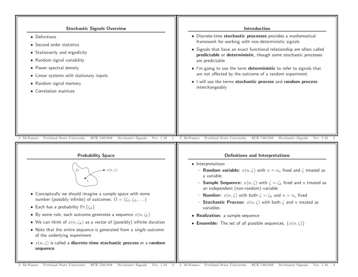
x(n, ζ) ζ Ω

• Conceptually we should imagine a sample space with some

number (possibly infinite) of outcomes: Ω = {ζ1, ζ2, . . . }

• Each has a probability Pr {ζk}
• By some rule, each outcome generates a sequence x(n, ζk)
• We can think of x(n, ζk) as a vector of (possibly) infinite duration
• Note that the entire sequence is generated from a single outcome
• f the underlying experiment
• x(n, ζ) is called a discrete-time stochastic process or a random

sequence

• J. McNames

Portland State University ECE 538/638 Stochastic Signals

• Ver. 1.10

3

Stochastic Signals Overview

• Definitions
• Second order statistics
• Stationarity and ergodicity
• Random signal variability
• Power spectral density
• Linear systems with stationary inputs
• Random signal memory
• Correlation matrices
• J. McNames

Portland State University ECE 538/638 Stochastic Signals

• Ver. 1.10

1

Definitions and Interpretations

• Interpretations

– Random variable: x(n, ζ) with n = no fixed and ζ treated as a variable – Sample Sequence: x(n, ζ) with ζ = ζk fixed and n treated as an independent (non-random) variable – Number: x(n, ζ) with both ζ = ζk and n = no fixed – Stochastic Process: x(n, ζ) with both ζ and n treated as variables

• Realization: a sample sequence
• Ensemble: The set of all possible sequences, {x(n, ζ)}
• J. McNames

Portland State University ECE 538/638 Stochastic Signals

• Ver. 1.10

4

Introduction

• Discrete-time stochastic processes provides a mathematical

framework for working with non-deterministic signals

• Signals that have an exact functional relationship are often called

predictable or deterministic, though some stochastic processes are predictable

• I’m going to use the term deterministic to refer to signals that

are not affected by the outcome of a random experiment

• I will use the terms stochastic process and random process

interchangeably

• J. McNames

Portland State University ECE 538/638 Stochastic Signals

• Ver. 1.10

2

SLIDE 2

Cross-Correlation and Cross-Covariance Cross-Correlation rxy(n1, n2) = E[x(n1)y∗(n2)] Cross-Covariance γxy(n1, n2) = E

• (x(n1) − µx(n1)) (y(n2) − µy(n2))∗

= rxy(n1, n2) − µx(n1)µ∗

y(n2)

Normalized Cross-Correlation ρxy(n1, n2) = γxy(n1, n2) σx(n1)σy(n2)

• J. McNames

Portland State University ECE 538/638 Stochastic Signals

• Ver. 1.10

7

Probability Functions In order to fully characterize a stochastic process, we must consider the cdf or pdf Fx(x1, . . . , xk; n1, . . . , nk) = Pr {x(n1) ≤ x1, . . . , x(nk) ≤ xk} fx(x1, . . . , xk; n1, . . . , nk) = ∂kFx(x1, . . . , xk; n1, . . . , nk) ∂x1 . . . ∂xk for every k ≥ 1 and any set of sample times {n1, n2, . . . , nk}.

• Without additional sweeping assumptions, estimation of fx(·)

from a realization is impossible

• Many stochastic processes can be characterized accurately or, at

least, usefully by much less information

• To simplify notation, from here on will mostly use x(n) to denote

both random processes and single realizations

• In most cases will assume x(n) is complex valued
• J. McNames

Portland State University ECE 538/638 Stochastic Signals

• Ver. 1.10

5

More Definitions

• Independent: iff

fx(x1, . . . , xk; n1, . . . , nk) =

k

• ℓ=1

fℓ(xℓ, ; nℓ) ∀k

• Uncorrelated: if

γx(n1, n2) =

• σ2

x(n1)

n1 = n2 n1 = n2

• Orthogonal: if

rx(n1, n2) =

• σ2

x(n1) + |µx(n1)|2

n1 = n2 n1 = n2

• J. McNames

Portland State University ECE 538/638 Stochastic Signals

• Ver. 1.10

8

Second Order Statistics At any time n, we can specify the mean and variance of x(n) µx(n) E[x(n)] σ2

x(n) E[|x(n) − µx(n)|2]

• µx(n) and σ2

x(n) are both deterministic sequences

• The expectation is taken over the ensemble.
• In general, the second-order statistics at two different times are

given by the autocorrelation or autocovariance sequences.

• Autocorrelation Sequence

rxx(n1, n2) = E[x(n1)x∗(n2)]

• Autocovariance Sequence

γxx(n1, n2) = E[(x(n1) − µx(n1)) (x(n2) − µx(n2))∗] = rxx(n1, n2) − µx(n1)µ∗

x(n2)

• J. McNames

Portland State University ECE 538/638 Stochastic Signals

• Ver. 1.10

6

SLIDE 3

Wide Sense Stationary fx(x1, x2; n1, n2) = fx(x1, x2; n1 + k, n2 + k)

• Wide-Sense Stationary (WSS): A stochastic process with a

constant mean and autocorrelation that only depends on the delay between the two sample times

• WSS Properties

E[x(n)] = µx rx(n1, n2) = rx(ℓ) = rx(n1 − n2) = E[x(n + ℓ)x∗(n)] γx(ℓ) = rx(ℓ) − |µx|2

• This implies the variance is also constant, var[x(n)] = σ2

x

• All processes that are stationary of order 2 are WSS
• Not all WSS processes are stationary of order 2
• Note this is slightly different from the text
• J. McNames

Portland State University ECE 538/638 Stochastic Signals

• Ver. 1.10

11

Still More Definitions

• Wide-sense Periodic: if

µx(n) = µx(n + N) ∀n rx(n1, n2) = rx(n1 + N, n2) = rx(n1, n2 + N) = rx(n1 + N, n2 + N)

• Statistically Independent: iff for every n1 and n2

fxy(x, y; n1, n2) = fx(x; n1)fy(y; n2)

• Uncorrelated: if for every n1 and n2,

γxy(n1, n2) = 0

• Orthogonal: if for every n1 and n2

rxy(n1, n2) = 0

• J. McNames

Portland State University ECE 538/638 Stochastic Signals

• Ver. 1.10

9

Example 1: Stationarity Describe a random process that is stationary. Describe a second random process that is not stationary.

• J. McNames

Portland State University ECE 538/638 Stochastic Signals

• Ver. 1.10

12

Stationarity Stationarity of Order N: A stochastic process x(n) such that fx(x1, . . . , xN; n1, . . . , nN) = fx(x1, . . . , xN; n1 + k, . . . , nN + k) for any value for any k.

• Any stochastic process of Order N, is also a stochastic process of
• rder M for all M ≤ N
• Strict-Sense Stationary (SSS): A stochastic process that is

stationary of all orders N

• J. McNames

Portland State University ECE 538/638 Stochastic Signals

• Ver. 1.10

10

SLIDE 4

Comments on Stationarity

• Many real processes are nonstationary
• Best case: can determine from domain knowledge of the process
• Else: must rely on statistical methods
• Many nonstationary processes are approximately locally stationary

(stationary over short periods of time)

• Much of time-frequency analysis is dedicated to this type of signal
• There is no general mathematical framework for analyzing

nonstationary signals

• However, many nonstationary stochastic processes can be

understood through linear estimation (i.e., Kalman filters)

• Note that nonstationary is a negative definition: not stationary
• J. McNames

Portland State University ECE 538/638 Stochastic Signals

• Ver. 1.10

15

Stationarity Notes

• SSS implies WSS
• If the marginal pdf of a signal is Guassian for all n, then WSS

implies SSS

• The book states that most WSS processes are SSS. True?
• Jointly Wide-Sense Stationary: two random signals x(n) and

y(n) are jointly WSS if they are both WSS and rxy(ℓ) = rxy(n1 − n2) = rxy(ℓ) = E[x(n)y∗(n − ℓ)] γxy(ℓ) = γxy(n1 − n2) = γxy(ℓ) = rxy(ℓ) − µxµ∗

y

• WSS is a very useful property because it enables us to consider a

spectral description

• In practice, we only need the signal to be WSS long enough to

estimate the autocorrelation or cross-correlation

• J. McNames

Portland State University ECE 538/638 Stochastic Signals

• Ver. 1.10

13

Introduction to Ergodicity

• In most practical situations we can only observe one or a few

realizations

• If the process is ergodic, we can know all statistical information

from a single realization

• Ensemble Averages: Repeat the experiment many times
• Time Averages:

(·) lim

N→∞

1 2N + 1

N

• n=−N

(·)

• J. McNames

Portland State University ECE 538/638 Stochastic Signals

• Ver. 1.10

16

Autocorrelation Sequence Properties rx(0) = σ2

x + |µx|2

rx(0) ≥ |rx(ℓ)| rx(ℓ) = r∗

x(−ℓ) M

• k=1

M

• m=1

αkrx(k − m)α∗

m

≥ ∀α sequences

• Average DC Power: |µx|2
• Average AC Power: σ2

x

• Nonnegative Definite: A sequence is said to be nonnegative

definite if it satisfies this last property

• Positive Definite: Any sequence that satisfies the last inequality

strictly for any α

• J. McNames

Portland State University ECE 538/638 Stochastic Signals

• Ver. 1.10

14

SLIDE 5

More on Ergodicity

• Joint Ergodicity: two random signals are jointly ergodic iff they

are individually ergodic and x(n)y∗(n − ℓ) = E[x(n)y∗(n − ℓ)]

• Stationarity ensures time invariance of the statistics
• Ergodicity implies the statistics can be obtained from a single

realization with time averaging

• In words: one realization (a single ζk) is sufficient to estimate any

statistic of the underlying random process

• J. McNames

Portland State University ECE 538/638 Stochastic Signals

• Ver. 1.10

19

Time Averages of Interest Mean value = x(n) Mean square = |x(n)|2 Variance = |x(n) − x(n)|2 Autocorrelation = x(n)x∗(n − ℓ) Autocovariance = [x(n) − x(n)][x(n − ℓ) − x(n)]∗ Cross-correlation = x(n)y∗(n − ℓ) Cross-covariance = [x(n) − x(n)][y(n − ℓ) − y(n)]∗

• Similar to correlation sequences for deterministic power signals
• Both quantitites have the same properties
• Difference

– Time averages are random variables (functions of the experiment outcome) – In the deterministic case the quantities are fixed numbers

• J. McNames

Portland State University ECE 538/638 Stochastic Signals

• Ver. 1.10

17

Problems with Ergodicity

• Problem we never know x(n) for n = −∞ to +∞
• In all real sitations, we only have finite records
• The most common estimator is then

(·)N 1 2N + 1

N

• n=−N

(·)

• Note that it is a random variable
• How good is it?

– Bias – Variance – Consistent – Confidence intervals – Distribution

• This is one of the key topics of this class
• J. McNames

Portland State University ECE 538/638 Stochastic Signals

• Ver. 1.10

20

Ergodic Random Processes

• Ergodic Random Process: a random signal for which the

ensemble averages equal the corresponding time averages

• Like stationarity, there are various degrees
• Ergodic in the Mean: a random process such that

x(n) = E[x(n)] = µx

• Ergodic in Correlation: a random process such that

x(n)x∗(n − ℓ) = E[x(n)x∗(n − ℓ)] = rx(ℓ)

• If a process is ergodic in both mean and correlation, it is also WSS
• Only stationary signals can be ergodic
• WSS does not imply any type of ergodicity
• Text: “Almost all stationary processes are also ergodic” True?
• Our usage: ergodic = ergodic in both the mean and correlation
• J. McNames

Portland State University ECE 538/638 Stochastic Signals

• Ver. 1.10

18

SLIDE 6

Periodic and Non-Periodic Processes Rx(ejω) F {rx(ℓ)} =

∞

• ℓ=−∞

rx(ℓ)e−jωℓ

• If rx(ℓ) is periodic, the DTFS is most appropriate
• Line Spectrum If we allow impulses in the PSD, then the PSD of

a periodic rx(ℓ) consists of an impulse train

• If the process x(n) is non-zero mean (i.e., nonzero average DC

power), the PSD will contain an impulse at ω = 0

• More generally, a random process can be composed of both

deterministic components and non-periodic components

• J. McNames

Portland State University ECE 538/638 Stochastic Signals

• Ver. 1.10

23

Ergodic Processes vs. Deterministic Signals rx(ℓ) = lim

N→∞

1 2N + 1

N

• n=−N

x(n)x∗(n − ℓ)

• The autocorrelation of a deterministic power signal and a ergodic

process can be calculated with the same infinite summation

• What’s the difference then?

– With deterministic signals there is only one signal – With stochastic signals, we assume it was generated from an underlying random experiment ζk – This enables us to consider the ensemble of possible signals: rx(ℓ) = E[x(n)x∗(n − ℓ)] – We can therefore draw inferences and make predictions about the population of possible outcomes, not merely this one signal

• Whether you define a given signal as deterministic or as a single

realization of a random process depends largely on the application

• J. McNames

Portland State University ECE 538/638 Stochastic Signals

• Ver. 1.10

21

Power Spectral Density Properties

• Rx(ejω) is real-valued
• Rx(ejω) is periodic with period 2π
• Rx(ejω) ≥ 0 is nonnegative definite
• Rx(ejω) has nonnegative area and

1 2π π

−π

Rx(ejω) dω = rx(0) = E[|x(n)|2]

• If x(n) is real-valued

– rx(ℓ) is real and even – Rx(ejω) is an even function of ω

• What if x(n) is complex-valued?
• J. McNames

Portland State University ECE 538/638 Stochastic Signals

• Ver. 1.10

24

Random Processes in the Frequency Domain Power Spectral Density (PSD) Rx(ejω)

• F {rx(ℓ)} =

∞

• ℓ=−∞

rx(ℓ)e−jωℓ rx(ℓ) = F−1 Rx(ejω)

• = 1

2π π

−π

Rx(ejω)ejω dω

• Stationary random processes have deterministic correlation

sequences

• They have a single index (independent variable)
• Note again that the power spectral density can be calculated with

the same equation for deterministic and ergodic signals

• J. McNames

Portland State University ECE 538/638 Stochastic Signals

• Ver. 1.10

22

SLIDE 7

Harmonic Process PSD x(n) =

M

• k=1

ak cos(ωkn + φk) ωk = 0

• The PSD consists of pairs of impulses (line spectrum) of area πa2

k

2

located a frequencies ±ωk Rx(ejω) = π 2

M

• k=1

a2

k [δ(ω − ωk) + δ(ω + ωk)]

− π ≤ ω ≤ π

• If all ωk/(2π) are rational numbers, x(n) is periodic and the

impulses are equally spaced apart

• This never happens, unless there is a single periodic (perhaps

non-sinusoidal) component

• Otherwise they are almost periodic (always happens)
• J. McNames

Portland State University ECE 538/638 Stochastic Signals

• Ver. 1.10

27

White Noise White Noise Process: A random WSS sequence w(n) such that E[w(n)] = µw rw(ℓ) =

• σ2

w + µ2 w

• δ(ℓ)
• Specifically, this is a second-order white process
• Notation: w(n) ∼ WN(µw, σ2

w)

• Not a complete characterization of w(n): the marginal pdf could

be anything

• If w(n) is Gaussian, then a white Guassian process is denoted by

w(n) ∼ WGN(µw, σ2

w)

• The term white comes from properties of white light
• J. McNames

Portland State University ECE 538/638 Stochastic Signals

• Ver. 1.10

25

Harmonic Process Comments x(n) =

M

• k=1

ak cos(ωkn + φk) ωk = 0

• It is only stationary if all of the random phases are equally likely

(uniformly distributed over all possible angles)

• This is an unusual circumstance where the signal is stationary but

is parameterized by one or more random variables that are constant over all n

• In general, is non-Guassian
• Is a predictable random sequence! (also highly unusual)
• J. McNames

Portland State University ECE 538/638 Stochastic Signals

• Ver. 1.10

28

Harmonic Process Harmonic Process any process defined by x(n) =

M

• k=1

ak cos(ωkn + φk) ωk = 0 where M, {ak}M

1 , and {ωk}M 1

are constant. The random variables {φk}M

1

are pairwise independent and uniformly distributed in the interval [−π, π].

• x(n) is stationary and ergodic with zero mean and autocorrelation

rx(ℓ) = 1

2 M

• k=1

a2

k cos(ωkℓ)

• Note the cosines in the autocorrelation are in-phase
• J. McNames

Portland State University ECE 538/638 Stochastic Signals

• Ver. 1.10

26

SLIDE 8

Linear Transforms and Coherence H(z)

x(n) y(n)

• Linear transforms have no effect on coherence
• Similar to the case of random variables: y = mx + b

– x and y are perfectly correlated: ρ = ±1

• J. McNames

Portland State University ECE 538/638 Stochastic Signals

• Ver. 1.10

31

Cross-Power Spectral Density Cross-power Spectral Density: if x(n) and y(n) are jointly stationary stochastic processes, Rxy(ejω)

• F {rxy(ℓ)} =

∞

• ℓ=−∞

rxy(ℓ)e−jωℓ rxy(ℓ) = 1 2π π

−π

Rxy(ejω)ejωℓ dω Rxy(ejω) = R∗

yx(ejω)

• Also known as the cross-spectrum
• Note that unlike the PSD, it is not real-valued, in general
• J. McNames

Portland State University ECE 538/638 Stochastic Signals

• Ver. 1.10

29

Linear Transforms and Coherence G(z)

w(n) x(n)

H(z) F(z)

y(n)

• G2

xy(ejω) =

Rx(ejω)|H(ejω)|2 Rx(ejω)|H(ejω)|2 + Rw(ejω)|G(ejω)|2

• Noise w(n) decreases coherence
• The final linear transform F(z) has no effect!
• J. McNames

Portland State University ECE 538/638 Stochastic Signals

• Ver. 1.10

32

Coherence Normalized Cross-Spectrum Gxy(ejω) Rxy(ejω)

• Rx(ejω)Ry(ejω)

Also known as the coherency spectrum or simply coherency. Similar to the correlation coefficient in frequency. Coherence Function G2

xy(ejω)

|Rxy(ejω)|2 Rx(ejω)Ry(ejω) Also known as the coherence and magnitude square coherence.

• If y(n) = h(n) ∗ x(n), then G2

xy(ejω) = 1

∀ω

• If rxy(ℓ) = 0, then G2

xy(ejω) = 0

∀ω

• 0 ≤ G2

xy ≤ 1

• J. McNames

Portland State University ECE 538/638 Stochastic Signals

• Ver. 1.10

30

SLIDE 9

Linear System Statistics h(n)

x(n) y(n)

H(z)

x(n) y(n)

Let x(n) be a random process that is the input to an LTI system with an output y(n). µy =

∞

• k=−∞

h(k) E[x(n − k)] = µx

∞

• k=−∞

h(k) = µxH(ej0) rxy(ℓ) =

∞

• k=−∞

h∗(k)rx(ℓ + k) =

∞

• m=−∞

h∗(−m)rx(ℓ − m) rxy(ℓ) = h∗(−ℓ) ∗ rx(ℓ) ryx(ℓ) = h(ℓ) ∗ rx(ℓ) ry(ℓ) = h(ℓ) ∗ rxy(ℓ) = h(ℓ) ∗ h∗(−ℓ) ∗ rx(ℓ) = rh(ℓ) ∗ rx(ℓ)

• J. McNames

Portland State University ECE 538/638 Stochastic Signals

• Ver. 1.10

35

Complex Spectral Density Functions Complex Spectral Density Rx(z) =

∞

• k=−∞

rx(ℓ)z−ℓ Ry(z) =

∞

• k=−∞

ry(ℓ)z−ℓ Complex Cross-Spectral Density Rxy(z) =

∞

• k=−∞

rxy(ℓ)z−ℓ

• J. McNames

Portland State University ECE 538/638 Stochastic Signals

• Ver. 1.10

33

Output Power h(n)

x(n) y(n)

H(z)

x(n) y(n)

Let x(n) be a random process that is the input to an LTI system with an output y(n). Py = ry(0) = [rh(ℓ) ∗ rx(ℓ)]ℓ=0 =

∞

• k=−∞

rh(k)rx(−k) =

∞

• k=−∞

rh(k)r∗

x(k)

If the system is FIR, then Py = hHRxh If µx = 0, then µy = 0 and σ2

y = Py

• J. McNames

Portland State University ECE 538/638 Stochastic Signals

• Ver. 1.10

36

Random Processes and Linear Systems If the input to an LTI system is a random process, so is the output. y(n, ζ) =

∞

• k=−∞

h(k)x(n − k, ζ)

• If the system is BIBO stable and the input process is stationary

with E[|x(n, ζ)|] < ∞, then the output converges absolutely with probability one.

• In English, the output is stationary
• If E[|x(n, ζ)|2] < ∞, then E[|y(n, ζ)|2] < ∞
• If the h(n) has finite energy, the output converges in the mean

square sense

• J. McNames

Portland State University ECE 538/638 Stochastic Signals

• Ver. 1.10

34

SLIDE 10

Frequency Domain Analysis h(n)

x(n) y(n)

H(z)

x(n) y(n)

If the system is stable, z = ejω lies in the ROC and the following relations hold Rxy(ejω) = H∗(ejω)Rx(ejω) Ryx(ejω) = H(ejω)Rx(ejω) Ry(ejω) = |H(ejω)|2Rx(ejω)

• Knowing ry(ℓ) and rx(ℓ) or the input and output PSD’s are

sufficient to determine |H(ejω)|

• We can’t estimate ∡H(ejω) from this information (the second
• rder statistics)
• Only rxy(ℓ) or Rxy(ejω) can provide phase information
• J. McNames

Portland State University ECE 538/638 Stochastic Signals

• Ver. 1.10

39

Output Distribution h(n)

x(n) y(n)

H(z)

x(n) y(n)

• In general, it is very difficult to solve for the output PDF (even

when y(n) is WSS)

• If x(n) is a Gaussian process, the output is a Gaussian process
• If x(n) is IID,

– The output is a weighted sum of IID random variables – If the distribution of x(n) is stable, then y(n) has the same distribution (even if the mean and variance differ) – If many of the largest weights are approximately equal so that many elements of the input signal have an equal effect on the

• utput, then the CLT applies (approximately) and the output

will be approximately Gaussian

• J. McNames

Portland State University ECE 538/638 Stochastic Signals

• Ver. 1.10

37

Random Signal & System Memory h(n)

x(n) y(n)

H(z)

x(n) y(n)

• Zero-memory: a process for which rx(ℓ) = σ2

xδ(ℓ)

• Examples: white noise, IID process
• We can create a signal with memory (dependence) by passing a

zero-memory process through an LTI system

• Extent and degree of imposed dependence depend on h(n)
• J. McNames

Portland State University ECE 538/638 Stochastic Signals

• Ver. 1.10

40

z Domain Analysis h(n)

x(n) y(n)

H(z)

x(n) y(n)

Z {h∗(−n)} = H∗(z−∗) Rxy(z) = Z {h∗(−ℓ) ∗ rx(ℓ)} = H∗(z−∗)Rx(z) Ryx(z) = Z {h(ℓ) ∗ rx(ℓ)} = H(z)Rx(z) Ry(z) = H(z)H∗(z−∗)Rx(z) Note that if h(n) is real, then h∗(−n) = h(−n) h(−n)

Z

← → H(z−1)

• J. McNames

Portland State University ECE 538/638 Stochastic Signals

• Ver. 1.10

38

SLIDE 11

Long Memory Processes

• Long memory: for WSS signal x(n) with finite variance, if there

exists 0 < α < 1 and Cr > 0 lim

ℓ→∞

1 Crσ2

x

rx(ℓ)ℓ−α = 1

• Equivalently, there exists 0 ≤ β < 1 and Cr > 0 such that

lim

ω→0

1 Crσ2

x

Rx(ejω)|ω|β = 1

• Implies

– The autocorrelation has heavy tails – Autocorrelation decays as a power law

∞

• ℓ=−∞

ρx(ℓ) = ∞ ρx(ℓ) ≈ Cr|ℓ|−α as ℓ → ∞ – Has infinite autocorrelation length

• J. McNames

Portland State University ECE 538/638 Stochastic Signals

• Ver. 1.10

43

Correlation Length

• Correlation Length: given a WSS process,

Lc = 1 rx(0)

∞

• ℓ=0

rx(ℓ) =

∞

• ℓ=0

ρx(ℓ)

• Equal to the “area” of the normalized autocorrelation curve
• Undesirable properties

– Why is it one sided? – Lengths should not be negative, in general. Could this be negative? r(ℓ) = [1.0000, −0.3214, −0.7538] for ℓ = 1, 2, 3 – “zero-memory” processes have a non-zero correlation length (Lc = 1)

• J. McNames

Portland State University ECE 538/638 Stochastic Signals

• Ver. 1.10

41

Correlation Matrices Let the random vector x(n) be related to the (possibly nonstationary) random process x(n) as follows x(n)

• x(n)

x(n − 1) · · · x(n − M + 1)H E[x(n)] = µx(n) µx(n − 1) · · · µx(n − M + 1)H Rx(n) = E[x(n)x(n)H] = ⎡ ⎢ ⎣ rx(n, n) · · · rx(n, n − M + 1) . . . ... . . . rx(n − M + 1, n) · · · rx(n − M + 1, n − M + 1) ⎤ ⎥ ⎦ Note that Rx(n) is nonnegative definite and Hermitian since rx(n − i, n − j) = r∗

x(n − j, n − i).

• J. McNames

Portland State University ECE 538/638 Stochastic Signals

• Ver. 1.10

44

Short Memory Processes

• Short Memory: a WSS process x(n) such that

∞

• ℓ=−∞

ρx(ℓ) < ∞

• For example, autocorrelation decays exponentially

ρx(ℓ) ≈ a|ℓ| for large ℓ

• J. McNames

Portland State University ECE 538/638 Stochastic Signals

• Ver. 1.10

42

SLIDE 12

Correlation Matrices If x(n) is a stationary process, the correlation matrix becomes Rx(n) = ⎡ ⎢ ⎢ ⎢ ⎢ ⎢ ⎣ rx(0) rx(1) rx(2) · · · rx(M − 1) r∗

x(1)

rx(0) rx(1) · · · rx(M − 2) r∗

x(2)

r∗

x(1)

rx(0) · · · rx(M − 3) . . . . . . . . . ... . . . r∗

x(M − 1)

r∗

x(M − 2)

r∗

x(M − 3)

· · · rx(0) ⎤ ⎥ ⎥ ⎥ ⎥ ⎥ ⎦ In this case Rx is Hermitian, Rx = RH

x , Toeplitz (the elements along

each diagonal are equal), and nonnegative definite.

• J. McNames

Portland State University ECE 538/638 Stochastic Signals

• Ver. 1.10

45

Conditioning of Correlation Matrix

• Condition number: of a positive definite matrix Rx is

χ(Rx) λmax λmin where λmax and λmin are the largest and smallest eigenvalues of the autocorrelation matrix, respectively

• If x(n) is a WSS random process, then the eigenvalues of the

autocorrelation matrix are bounded by the dynamic range of the PSD min

ω R(ejω) ≤ λi ≤ max ω

R(ejω) ∀λi

• See text for proof
• Interpretation: a large spread in eigenvalues implies

– PSD is more variable (less flat) – Process is less like white nose (more predictable)

• J. McNames

Portland State University ECE 538/638 Stochastic Signals

• Ver. 1.10

46