Zeros of random analytic functions and extreme value theory Zakhar - - PowerPoint PPT Presentation

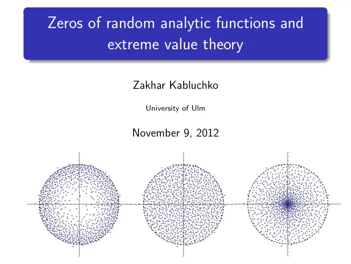
Zeros of random analytic functions and extreme value theory

Zakhar Kabluchko

University of Ulm

November 9, 2012

A random equation

Statement of the problem We consider an algebraic equation with random coefficients, for example z2000 − z1999 + z1998 + z1997 − z1996 − . . . + z3 + z2 − z + 1 = 0 What is the distribution of the solutions of this equation in the complex plane?

2

Solutions of the equation

Zeros of a random polynomial of degree n = 2000

3

Random Polynomials (Kac Ensemble)

Statement of the problem Let ξ0, ξ1, . . . be i.i.d. random variables. Consider the equation Pn(z) := ξ0 + ξ1z + ξ2z2 + . . . + ξnzn = 0. The equation has n complex roots z1, . . . , zn. What is the distribution of roots in the complex plane? Consider the empirical measure µn = 1 n

n

• k=1

δ(zk). Problem: Find limn→∞ µn.

4

Distribution of roots

Theorem (Ibragimov, Zaporozhets, 2011) The following conditions are equivalent:

1 With probability 1, the sequence µn converges weakly to

the uniform distribution on the unit circle.

2 E log(1 + |ξ0|) < ∞.

Remark The series ∞

k=0 ξkzk converges a.s. in the unit circle iff

E log(1 + |ξ0|) < ∞. History Hammersley (1954), Shparo und Shur (1962), Arnold (1966), Shepp und Vanderbei (1995), ...

5

Logarithmic tails

Problem What happens if the coefficients ξk are heavy-tailed? Logarithmic tails We consider coefficients satisfying P[|ξ0| > t] ∼ L(log t) (log t)α , t → +∞, where α > 0 and L is a slowly varying function. Remark E log(1 + |ξ0|) is

• infinite,

α < 1, finite, α > 1.

6

Example: Coefficients with logarithmic tails

The coefficients ξk are such that P[|ξk| > t] = 1/(log t)2 and the degree is n = 2000.

7

Distribution of roots

Assume for simplicity that P[|ξ0| > t] ∼ 1 (log t)α as t → +∞. (1) Theorem (Kabluchko, Zaporozhets, 2011) For coefficients with logarithmic tails, the following weak con- vergence of random probability measures holds: 1 n

n

• k=1

δ(zn1− 1

α

k

)

w

− →

n→∞ Πα.

The limiting random probability measure Πα is a.s. a convex combination of at most countably many uniform measures con- centrated on circles centered at the origin.

8

Light and logarithmically tailed coefficients

9

Distribution of roots

Example: α = 1 If P[|ξ0| > t] ∼

1 log t as t → +∞, then we have

1 n

n

• k=1

δ(zk)

w

− →

n→∞ Π1.

No normalization of roots is needed. Example: α > 1 (E log |ξ0| < ∞) The roots approach the unit circle. The distance between the roots and the unit circle is of order n

1 α −1.

Example: α < 1 (E log |ξ0| = ∞) The roots diverge to ∞ and 0. The absolute values of the roots are of order O(1)n

1 α −1. 10

Extremal order statistics of the coefficients

Theorem Let ξ0, ξ1, . . . be i.i.d. random variables with P[log |ξk| > t] ∼ t−α as t → +∞. Then, we have the following weak convergence of point pro- cesses on [0, 1] × (0, ∞):

n

• k=0

δ k n, log |ξk| n1/α

• w

− →

n→∞ PPP

• αv −(α+1)dudv
• .

11

Extremal order statistics of the coefficients

12

Newton polygon

Idea of the proof For large n consider the equation ±enx1 ± . . . ± enxd = 0, where xi > 0. The most easy way for this to be true is the following:

1 Two terms, say enxk and enxl, cancel each other. 2 All other terms are much smaller than these two. 13

Newton polygon

Idea of the proof Apply this to the equation ξ0 + ξ1z + . . . + ξnzn = 0.

1 Two terms cancel each other: ξkzk + ξlzl = 0. 2 All other terms are much smaller than these two.

Geometrically: the points (k, log |ξk|) and (l, log |ξl|) are neigh- boring vertices of the least concave majorant of the set {(0, log |ξ0|), . . . , (n, log |ξn|)}.

14

The least concave majorant

Remark The number of segments is finite a.s. if and only if α < 1.

15

Limiting empirical measure of the roots

Limiting measure Πα Consider the least concave majorant of the Poisson process with intensity αv −(α+1)dudv.

1 Radii of circles = exponentials of the slopes of the majo-

rant.

2 Number of roots on a circle = length of the linearity inter-

val.

16

Very heavy tails: α = 0

Let the coefficients be such that P[|ξ0| > t] ∼ L(log t) as t → +∞, where L is a slowly varying function. The roots concentrate on two circles, one with a small radius,

• ne with a large radius. The proportion of the roots lying on

the small circle is uniform on [0, 1].

17

Weyl Polynomials

Let ξ0, ξ1, . . . be i.i.d. random variables. Consider the Weyl Polynomials Pn(z) =

n

• k=0

ξk zk √ k! . Let z1, . . . , zn be the zeros of Pn. Theorem (Kabluchko, Zaporozhets, 2012) The following conditions are equivalent:

1 The sequence of probability measures 1

n

• k=1 δ( zk

√n) con-

verges a.s. to the uniform distribution on the unit disk {|z| ≤ 1}.

2 E log(1 + |ξ0|) < ∞. 18

Weyl Polynomials

Zeros of a Weyl polynomial: Normally distributed coefficients

19

Weyl Polynomials

Zeros of a Weyl polynomial: Logarithmic tails

20

Littlewood–Offord Polynomials (1939)

Let ξ0, ξ1, . . . be i.i.d. random variables with E log(1 + |ξ0|) < ∞. Consider the Littlewood–Offord polynomials Pn(z) =

n

• k=0

ξk zk (k!)α. Let z1, . . . , zn be the zeros of Pn. Theorem (Kabluchko, Zaporozhets, 2012) With probability 1, the sequence

• f

random measures

1 n

n

k=1 δ( zk nα) converges to the probability measure with the

density 1 2πα|z|

1 α −2, |z| < 1. 21

Littlewood–Offord Polynomials

Zeros of the Littlewood–Offord polynomials: Normal coefficients

22

Littlewood–Offord Polynomials

Zeros of the Littlewood–Offord polynomials: Logarithmic coefficients

23

Szeg¨

• Polynomials

Szeg¨

• Polynomials: sn(z) = n

k=0 zk k!.

Theorem (Szeg¨

• , 1924)

The zeros of sn(nz) cluster along the curve |ze1−z| = 1, |z| < 1.

24

Zeros in the Random Energy Model

Random Energy Model (Derrida, 1981) A system has N states. The energy of the system in state i is √log Nξi. ξ1, . . . , ξN are i.i.d. standard Gaussian random variables. Consider the partition function ZN(β) =

N

• k=1

eβ√log Nξk, β ∈ C. Other motivations ZN is an empirical Laplace transform. ZN is a nice random analytic function.

25

Zeros in the Random Energy Model

Complex zeros of ZN. Source: C. Moukarzel und N. Parga: Physica A 177 (1991).

26

Zeros in the Random Energy Model

Theorem (Derrida, 1991) For β = σ + iτ ∈ C it holds that lim

N→∞

log |ZN(β)| log N =      1 + 1

2(σ2 − τ 2),

β ∈ B1, √ 2|σ|, β ∈ B2,

1 2 + σ2,

β ∈ B3, where B1 = C\B2 ∪ B3, B2 = {β ∈ C : 2σ2 > 1, |σ| + |τ| > √ 2}, B3 = {β ∈ C : 2σ2 < 1, σ2 + τ 2 > 1}.

27

Zeros in the Random Energy Model

Theorem (Derrida, 1991) The random measure 2π log N

• β:ZN(β)=0

δ(β) converges weakly (as N → ∞) to the deterministic measure Ξ = 2Ξ3 + Ξ12 + Ξ13. Here, Ξ3 is the Lebesgue measure on B3. Ξ13 is the one-dimensional Lebesgue measure on the boundary between B1 and B3. Ξ12 is the measure with density √ 2|τ| on the boundary between B1 and B2. Rigorous proof, further results: Kabluchko und Klimovsky, 2012.

28