
SLIDE 1
X-ray spectral timing: methods and interpretation
Phil Uttley
Why spectral-timing?
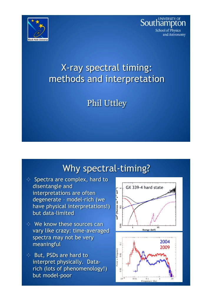
Spectra are complex, hard to
disentangle and interpretations are often degenerate – model-rich (we have physical interpretations!) but data-limited
We know these sources can
vary like crazy: time-averaged spectra may not be very meaningful
But, PSDs are hard to
interpret physically. Data- rich (lots of phenomenology!) but model-poor
2004 2009
GX 339-4 hard state