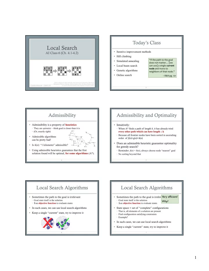
X Example? In such cases, we can use local search algorithms Keep - - PDF document

1

Local Search

AI Class 6 (Ch. 4.1-4.2)

Cynthia Matuszek – CMSC 671

Based on slides by Dr. Marie desJardin. Some material also adapted from slides by Dr. Matuszek @ Villanova University, which are based on Hwee Tou Ng at Berkeley, which are based on Russell at Berkeley. Some diagrams are based on AIMA.

Today’s Class

• Iterative improvement methods
• Hill climbing
• Simulated annealing
• Local beam search
• Genetic algorithms
• Online search

3

“If the path to the goal does not matter… [we can use] a single current node and move to neighbors of that node.” – R&N pg. 121

Admissibility

• Admissibility is a property of heuristics
• They are optimistic – think goal is closer than it is
• (Or, exactly right)
• Admissible algorithms

can be pretty bad!

• Is h(n): “1 kilometer” admissible?
• Using admissible heuristics guarantees that the first

solution found will be optimal, for some algorithms (A*).

4

Admissibility and Optimality

• Intuitively:
• When A* finds a path of length k, it has already tried

every other path which can have length ≤ k

• Because all frontier nodes have been sorted in ascending
• rder of f(n)=g(n)+h(n)
• Does an admissible heuristic guarantee optimality

for greedy search?

• Reminder: f(n) = h(n), always choose node “nearest” goal
• No sorting beyond that

5

E

Local Search Algorithms

6

• Sometimes the path to the goal is irrelevant
• Goal state itself is the solution
• an objective function to evaluate states
• In such cases, we can use local search algorithms
• Keep a single “current” state, try to improve it

X

E

Local Search Algorithms

7

• Sometimes the path to the goal is irrelevant
• Goal state itself is the solution
• an objective function to evaluate states
• State space = set of “complete” configurations
• That is, all elements of a solution are present
• Find configuration satisfying constraints
• Example?
• In such cases, we can use local search algorithms
• Keep a single “current” state, try to improve it

Very efficient! Why?

2

State Space (Landscape)

8

State Space (Landscape)

A B S S A 1 B 4

2

Iterative Improvement Search

• Start with an initial guess
• Gradually improve it until it is legal or optimal
• Some examples:
• Hill climbing
• Simulated annealing
• Constraint satisfaction

10

Hill Climbing on State Surface

• Concept:

trying to reach the “highest” (most desirable) point (state)

• “Height”

Defined by Evaluation Function

11

Hill Climbing Search

• If there exists a successor s for the current state n such that
• h(s) > h(n)
• h(s) >= h(t) for all the successors t of n,

then move from n to s. Otherwise, halt at n.

• Look one step ahead to determine if any successor is “better” than

current state

• If so, move to the best successor
• A kind of Greedy search in that it uses h
• But, does not allow backtracking or jumping to an alternative path
• Doesn’t “remember” where it has been.
• Not complete
• Search will terminate at local minima, plateaux, ridges.

12

2 8 3 1 6 4 7 5 2 8 3 1 4 7 6 5 2 3 1 8 4 7 6 5 1 3 8 4 7 6 5 2 3 1 8 4 7 6 5 2 1 3 8 4 7 6 5 2 start goal

• 5

h = -3 h = -3 h = -2 h = -1 h = 0 h = -4

• 5
• 4
• 4
• 3
• 2

f(n) = -(number of tiles out of place)

Hill Climbing Example

3

Image from: http://classes.yale.edu/fractals/CA/GA/Fitness/Fitness.html

local maximum ridge plateau

Exploring the Landscape

• Local Maxima:
• Peaks that aren’t the highest

point in the space

• Plateaus:
• A broad flat region that gives

the search algorithm no direction (random walk)

• Ridges:
• Flat like a plateau, but with

drop-offs to the sides; steps to the North, East, South and West may go down, but a step to the NW may go up.

Drawbacks of Hill Climbing

• Problems: local maxima, plateaus, ridges
• Remedies:
• Random restart: keep restarting the search from random

locations until a goal is found.

• Problem reformulation: reformulate the search space to

eliminate these problematic features

• Some problem spaces are great for hill climbing;
• thers are terrible

15

Example of a Local Optimum

1 2 5 8 7 4 6 3 4 1 2 3 8 7 6 5 1 2 5 8 7 4 3 f = -6 f = -7 f = -7 f = 0 start goal 2 5 7 4 8 6 3 1 6

move up move right

f = -(manhattan distance)

16

Some Extensions of Hill Climbing

• Simulated Annealing
• Escape local maxima by allowing some “bad” moves but

gradually decreasing their frequency

• Local Beam Search
• Keep track of k states rather than just one
• At each iteration:
• All successors of the k states are generated and evaluated
• Best k are chosen for the next iteration

17

Some Extensions of Hill Climbing

• Stochastic Beam Search
• Chooses semi-randomly from “uphill” possibilities
• “Steeper” moves have a higher probability of being chosen
• Random-Restart Climbing
• Can actually be applied to any form of search
• Pick random starting points until one leads to a solution
• Genetic Algorithms
• Each successor is generated from two predecessor (parent)

states

18

• Take downward “steps” proportional to the negative of the

gradient of the function at current state.

• “Steepest descent”
• Gradient descent procedure for finding the argx min f(x)
• choose initial x0 randomly
• repeat
• xi+1 xi – f’ (xi)
• until the sequence x0, x1, …, xi, xi+1 converges
• Step size(eta) is

small (~0.1–0.05)

• Good for differentiable, continuous spaces

Gradient Ascent / Descent

Images from http://en.wikipedia.org/wiki/Gradient_descent

19

4

Gradient Ascent / Descent

Images from http://en.wikipedia.org/wiki/Gradient_descent

20

Gradient Methods vs. Newton’s Method

• A reminder of Newton’s

method from Calculus: xi+1 xi – f’ (xi) / f’’ (xi)

• Newtons method uses 2nd
• rder information (the second

derivative, or, curvature) to take a more direct route to the minimum.

• The second-order information

is more expensive to compute, but converges more quickly.

Contour lines of a function (blue)

• Gradient descent (green)
• Newton’s method (red)

Images from http://en.wikipedia.org/wiki/Newton's_method_in_optimization

Simulated Annealing

• Simulated annealing (SA): analogy between the way

metal cools into a minimum-energy crystalline structure and the search for a minimum generally

• In very hot metal, molecules can move fairly freely
• But, they are slightly less likely to move out of a stable structure
• As you slowly cool the metal, more molecules are “trapped” in

place

• Conceptually: Escape local maxima by allowing some

“bad” (locally counterproductive) moves but gradually decreasing their frequency

22

Simulated Annealing (II)

• Can avoid becoming trapped at local minima.
• Uses a random local search that:
• Accepts changes that increase objective function f
• As well as some that decrease it
• Uses a control parameter T
• By analogy with the original application
• Is known as the system “temperature”
• T starts out high and gradually decreases toward 0

23

freedom to make “bad” moves

Simulated Annealing (IV)

• f (s) represents the quality of state n (high is good)
• A “bad” move from A to B is accepted with a probability

P(moveAB) ≈ e

( f (B) – f (A)) / T

• (Note that f (B) – f (A) will be negative, so bad moves always have a relative

probability less than one. Good moves, for which f (B) – f (A) is positive, have a relative probability greater than one.)

• Temperature
• Higher temperature = more likely to make a “bad” move
• As T tends to zero, this probability tends to zero
• SA becomes more like hill climbing
• If T is lowered slowly enough, SA is complete and admissible.
• domain-specific
• sometimes hard to determine

Local Beam Search

• Begin with k random states
• k, instead of one, current state(s)
• Generate all successors of these states
• Keep the k best states
• Stochastic beam search
• Probability of keeping a state is a function of its heuristic

value

• More likely to keep “better” successors

27

5

Genetic Algorithms

• The Idea:
• New states are generated by

“mutating” a single state or “reproducing” (somehow combining) two parent states

• Selected according to their fitness
• Similar to stochastic beam search
• Start with k random states (the initial population)
• Encoding used for the “genome” of an individual strongly affects the

behavior of the search

• Must have some combinable representation of state spaces
• Genetic algorithms / genetic programming are a large and active area
• f research

28

+

Tabu Search

• Problem: Hill climbing can get stuck on local

maxima

• Solution: Maintain a list of k previously visited

states, and prevent the search from revisiting them

• Why not always do this?

29

Online Search

• Interleave computation and action (search some, act some)
• Exploration: Can’t infer outcomes of actions; must actually perform them to learn what

will happen

• Competitive ratio = Path cost found* / Path cost that could be found**

* On average, or in an adversarial scenario (worst case) ** If the agent knew the nature of the space, and could use offline search

• Relatively easy if actions are reversible
• LRTA* (Learning Real-Time A*): Update h(s) (in state table) based on

experience

• More about online search and nondeterministic actions next time…

30

Summary: Informed Search (I)

• State space can be treated as a “landscape” of movement on quality of

states where we are trying to find “high” points

• Best-first search is a general search where the minimum-cost nodes are

expanded first.

• Greedy search uses minimal estimated cost h(n) to the goal state as

measure of goodness.

• Reduces search time, but is neither complete nor optimal.

31

Summary: Informed Search (II)

• Hill-climbing algorithms keep only a single state in memory, but can get

stuck on local optima.

• Simulated annealing escapes local optima, and is complete and optimal

given a “long enough” cooling schedule.

• Genetic algorithms search a space by modeling biological evolution.
• Online search algorithms are useful in state spaces with partial/no

information.

32

Questions?

Class Exercise: Local Search for N-Queens

Q Q Q Q Q Q (more on constraint satisfaction heuristics next time...)