[PPT] - Wiener Measure Heuristics and the Feynman-Kac formula Theorem 1 PowerPoint Presentation

SLIDE 1

Path integrals over Euclidean spaces

Bruce Driver

Visiting Miller Professor (Permanent Address) Department of Mathematics, 0112 University of California at San Diego, USA http://math.ucsd.edu/∼driver Student Topology Seminar University of California, Berkeley, August 29, 2007

Wiener Measure Heuristics and the Feynman-Kac formula

Theorem 1 (Trotter Product Formula). Let A and B be d × d matrices. Then

e(A+B) = lim

n→∞

e

A ne B n

n

. Proof: By the chain rule,

d dε|0 log(eεAeεB) = A + B.

Hence by Taylor’s theorem with remainder,

log(eεAeεB) = ε (A + B) + O

ε2

which is equivalent to

eεAeεB = eε(A+B)+O(ε2).

Taking ε = 1/n and raising the result to the nth – power gives

(en−1Aen−1B)n =

en−1(A+B)+O(n−2)n

= eA+B+O(n−1) → e(A+B) as n → ∞.

Q.E.D.

Bruce Driver 2 University of California, Berkeley, August 29, 2007

Fact (Trotter product formula). For “nice enough” V,

eT(∆/2−V ) = strong– lim

n→∞[e

T 2n∆e−T nV ]n.

(1) See [1] for a rigorous statement of this type. Lemma 2. Let V : Rd → R be a continuous function which is bounded from below, then

e

T n∆/2e−T nV n

f

(x0)

=

Rdn

pT

n(x0, x1)e−T nV (x1) . . . pT n(xn−1, xn)e−T nV (xn)f(xn)dx1 . . . dxn

= ⎛ ⎜ ⎝ 1

2πT

n

⎞ ⎟ ⎠

dn (Rd)n

e

− n

2T n

i=1

|xi−xi−1|2−T

n n

i=1

V (xi)

f(xn)dx1 . . . dxn.

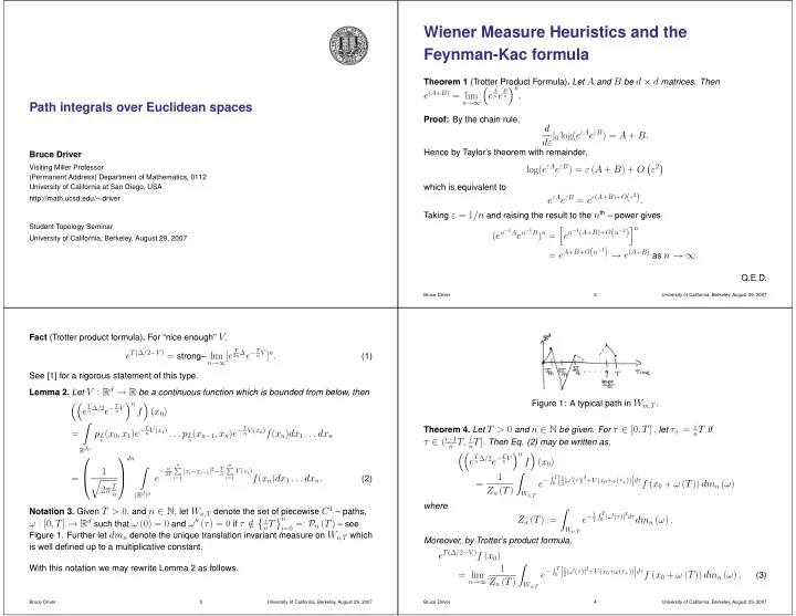
(2) Notation 3. Given T > 0, and n ∈ N, let Wn,T denote the set of piecewise C1 – paths,

ω : [0, T] → Rd such that ω (0) = 0 and ω′′ (τ) = 0 if τ / ∈ i

nT

n

i=0 =: Pn (T) – see

Figure 1. Further let dmn denote the unique translation invariant measure on Wn,T which is well defined up to a multiplicative constant. With this notation we may rewrite Lemma 2 as follows.

Bruce Driver 3 University of California, Berkeley, August 29, 2007

Figure 1: A typical path in Wm,T. Theorem 4. Let T > 0 and n ∈ N be given. For τ ∈ [0, T] , let τ+ = i

nT if

τ ∈ (i−1

n T, i nT]. Then Eq. (2) may be written as,

e

T n∆/2e−T nV n

f

(x0)

= 1 Zn (T)

Wn,T

e−

T

0 [1 2|ω′(τ)|2+V (x0+ω(τ+))]dτf (x0 + ω (T)) dmn (ω)

where

Zn (T) :=

Wn,T

e−1

2

T

0 |ω′(τ)|2dτdmn (ω) .

Moreover, by Trotter’s product formula,

eT(∆/2−V )f (x0) = lim

n→∞

1 Zn (T)

Wn,T

e−

T

0 [1 2|ω′(τ)|2+V (x0+ω(τ+))]dτf (x0 + ω (T)) dmn (ω) .

(3)

Bruce Driver 4 University of California, Berkeley, August 29, 2007

SLIDE 2

Following Feynman, at an informal level (see Figure 2), Wn,T → WT as n → ∞, where

WT :=

ω ∈ C
[0, T] → Rd

: ω (0) = 0

.

Moreover, formally passing to the limit in Eq. (3) leads us to the following heuristic Figure 2: A typical path in WT may be approximated better and better by paths in Wm,T as m → ∞. expression for

eT(∆/2−V )f
(x0) ;
eT(∆/2−V )f
(x0) = “

1 Z (T)

WT

e−

T

0 [1 2|ω′(τ)|2+V (x0+ω(τ))]dτf (x0 + ω (T)) Dω”

(4) where Dω is the non-existent Lebesgue measure on WT, and Z (T) is the

Bruce Driver 5 University of California, Berkeley, August 29, 2007

“normalization” constant (or partition function) given by

Z (T) = “

WT

e−1

2

T

0 |ω′(τ)|2dτDω.”

This expression may also be written in the Feynman – Kac form as

eT(∆/2−V )f (x0) =

WT

e−

T

0 V (x0+ω(τ))dτf (x0 + ω (T)) dµ (ω) ,

where

dµ (ω) = “ 1 Z (T)e−1

2

T

0 |ω′(τ)|2dτDω”

(5) is the informal expression for Wiener measure on WT. Thus our immediate goal is to make sense out of Eq. (5). Let

HT :=

h ∈ WT :

T |h′ (τ)|2 dτ < ∞

with the convention that

T

0 |h′ (τ)|2 dτ := ∞ if h is not absolutely continuous. Further let

h, kT := T h′ (τ) · k′ (τ) dτ for all h, k ∈ HT

and Xh (ω) := h, ωT for h ∈ HT. Since

dµ (ω) = “ 1 Z (T)e−1

2ω2 HTDω, ”

(6)

Bruce Driver 6 University of California, Berkeley, August 29, 2007

dµ (ω) should be a Gaussian measure on HT and hence we expect,

HT

eih,ωTdµ (ω) = exp

−1

2 h2

HT

.

(7)

Bruce Driver 7 University of California, Berkeley, August 29, 2007

Gaussian Measures “on” Hilbert spaces

Goal Given a Hilbert space H, we would ideally like to define a probability measure µ on

B(H) such that ˆ µ(h) :=

H

ei(λ,x)dµ(x) = e−1

2λ2 for all λ ∈ H

(8) so that, informally,

dµ (x) = 1 Ze−1

2|x|2 HDx.

(9) The next proposition shows that this is impossible when dim(H) = ∞. Proposition 5. Suppose that H is an infinite dimensional Hilbert space. Then there is no probability measure µ on B = B(H) such that Eq. (8) holds. Proof: Suppose such a Gaussian measure were to exist. Let {λi}∞

i=1 be an orthonormal

set in H and for M > 0 and n ∈ N let

W M

n = {x ∈ H : |(λi, x)| ≤ M for i = 1, 2, . . . , n}.

Let µn be the standard Gaussian measure on Rn,

dµn(y) = (2π)−n/2e−y·y/2dy.

Bruce Driver 8 University of California, Berkeley, August 29, 2007

SLIDE 3

Then for all bounded measurable functions f : Rn → R, we have

H

f((λ1, x), . . . , (λn, x)) dµ(x) =

Rn

f(y)dµn(y)

and therefore,

µ(W M

n ) = µn({y ∈ Rn : |yi| ≤ M for i = 1, . . . , n})

=

(2π)−1/2

M

−M

e−1

2y2dy

n → 0 as n → ∞.

Because

W M

n ↓ HM := {x ∈ H : |(λi, x)| ≤ M ∀ i = 1, 2, . . . },

µ(HM) = limn→∞ µ(W M

n ) = 0 for all M > 0. Since HM ↑ H as M ↑ ∞ we learn that

µ(H) = limM→∞ µ(HM) = 0, i.e. µ ≡ 0.

Q.E.D. Moral: The measure µ must be defined on a larger space. This is somewhat analogous to trying to define Lebesgue measure on the rational numbers. In each case the measure can only be defined on a certain completion of the naive initial space.

Bruce Driver 9 University of California, Berkeley, August 29, 2007

Guassian Measure for ℓ2

Remark 6. Suppose that H = ℓ2 the space of square summable sequences {xn}∞

n=1 . In

this case the Gaussian measure that we are trying to construct is formally given by the expression

dµ(x) = 1 ( √ 2π)∞ exp

−1

2Σ∞

i=1x2 i

∞
i=1

dxi =

∞

i=1

1 √ 2πe−1

2x2 i dxi

=:

∞

i=1

p1(dxi),

where p1(dx) is the heat kernel defined by

pt (x) = 1 √ 2πt exp

− 1

2tx2

.

This suggests that we define µ = p⊗N

1 , the infinite product measure on RN.

Theorem 7. Let µ = p⊗N

1

be the infinite product measure on

RN, F
where µ and F.

Also let a = (a1, a2, . . . ) ∈ (0, ∞)N be a sequence and define

Xa = ℓ2(a) = {x ∈ RN :

∞

i=1aix2 i := xa < ∞}.

Bruce Driver 10 University of California, Berkeley, August 29, 2007

So X = L2(N, a) where a now denotes the measure on N determined by a ({i}) = ai for all i ∈ N. Then Xa ∈ F, FXa := {A ∩ Xa : A ∈ F} = B(Xa) (B(Xa) is the Borel σ – field on Xa) and

µ(Xa) = ⎧ ⎨ ⎩ 1

if

∞

i=1

ai < ∞ 0 otherwise.

(10) Assuming that

∞

i=1

ai < ∞, µa := µ|B(Xa) is a the unique probability measure on (Xa, B(Xa)) which satisfies

Xa

f(x1, . . . , xn)dµa(x) =

Rn

f(x1, . . . , xn)p1(dxi) . . . p1(dxn)

(11) for all f ∈ (B(Rn))b and n = 1, 2, 3, . . . Proof: For N ∈ N, let qN : RN → R be defined by qN(x) = N

i=1aix2

i. Then it is easily

seen that qN is F – measurable. Therefore, q := supN∈N qN (also notice that qN ↑ q as

N → ∞) is F – measurable as well and hence Xa = {x ∈ RN : q(x) < ∞} ∈ F.

Similarly, if x0 ∈ Xa, then q(· − x0) = supN∈N qN(· − x0) is F – measurable and therefore for r > 0,

B(x0, r) = {x ∈ Xa : x − x0a < r} = {x ∈ RN : q(· − x0) < r2} ∈ F

Bruce Driver 11 University of California, Berkeley, August 29, 2007

which shows that B(Xa) ⊂ F and hence B(Xa) ⊂ FXa. To prove the reverse inclusion, let i : Xa → RN be the inclusion map and recall that

FXa = i−1 (F) = i−1 σ

π−1

j (B) : j ∈ N and B ∈ BR

= σ
i−1π−1

j (B) : j ∈ N and B ∈ BR

= σ
(πj ◦ i)−1 (B) : j ∈ N and B ∈ BR
= σ (πj ◦ i : j ∈ N) .

Since πj ◦ i ∈ X∗

a for all j, we see from this expression that

FXa ⊂ σ(X∗

a) = B(Xa).

Let us now prove Eq. (10). Letting q and qN be as defined above, for any ε > 0,

RN e−εq/2dµ =
RN lim

N→∞ e−εqN/2dµ

M.C.T.

= lim

N→∞

RN e−εqN/2dµ

= lim

N→∞

RN e

−ε

2 N

1

aix2

i

N

i=1

p1(dxi) = lim

N→∞ N

i=1
R

e−ε

2aix2p1(dx).

(12) Using

e−λ

2x2p1(x)dx =

1 √ 2π

e−λ+1

2 x2dx =

1 √ 2π

2π

λ + 1 = 1 √ λ + 1

Bruce Driver 12 University of California, Berkeley, August 29, 2007

SLIDE 4

in Eq. (12) we learn that

RN e−εq/2dµ = lim

N→∞ N

1

1 √1 + εai =

lim

N→∞ N

1

(1 + εai)−1

r equivalently that

− log

RN e−εq/2dµ
= 1

2

∞

i=1

ln(1 + εai).

(13) Notice that there is δ > 0 such that

ln(1 + x) ≤ x ∀x ≥ 0 and ln(1 + x) ≥ x/2 for x ∈ [0, δ].

(14) If lim supi→∞ ai = 0, then

∞

i=1

ln(1 + εai) = ∞ for all ε > 0. If limi→∞ ai = 0 but ∞

i=1 ai = ∞, then using Eq. (14), ln(1 + εai) ≥ εai/2 for all i large and hence again ∞

i=1

ln(1 + εai) = ∞. If ∞

i=1 ai < ∞ then by Eq. (14), ∞

i=1

ln(1 + εai) ≤ ε

∞

i=1

ai → 0 as ε ↓ 0.

Bruce Driver 13 University of California, Berkeley, August 29, 2007

In summary,

− lim

ε↓0 log

RN e−εq/2dµ
=

⎧ ⎨ ⎩ ∞ if ∞

i=1 ai = ∞

if ∞

i=1 ai < ∞

r equivalently,

lim

ε↓0

RN e−εq/2dµ =

⎧ ⎨ ⎩ 0 if ∞

i=1 ai = ∞

1 if ∞

i=1 ai < ∞.

Since e−εq/2 ≤ 1 and limε↓0 e−εq/2 = 1Xa, the previous equation along with the dominated convergence theorem shows that

µ(Xa) =

RN 1Xadµ =
0 if ∞

i=1 ai = ∞

1 if ∞

i=1 ai < ∞.

proving Eq. (10inally Eq. (11) follows from the definition of µ and the fact that

Xa

f(x1, . . . , xn)dµa(x) =

RN f(x1, . . . , xn)dµ(x).

Q.E.D.

Bruce Driver 14 University of California, Berkeley, August 29, 2007

Classical Wiener Measure

Let W = {ω ∈ C([0, 1] → R) : ω(0) = 0} and let H denote the set of functions h ∈ W which are absolutely continuous and satisfy (h, h) =

1

0 |h′(s)|2ds < ∞. The space H

is called the Cameron-Martin space and is a Hilbert space when equipped with the inner product

(h, k) = 1 h′(s)k′(s)ds for all h, k ∈ H.

The space W is a Banach space when equipped with the sup-norm,

f = max

x∈[0,1] |f(x)| .

Theorem 8 (Wiener, 1923). There exists a unique Gaussian measure µ on W such that

W

eiϕ(x)dµ(x) = e−q(ϕ)/2,

(15) where ϕ = (·, hϕ) , and q(ϕ, ψ) := (hϕ, hψ)H is the dual inner product to H. Theorem 9 (Feynman-Kac Formula). Suppose that V : Rd → R is a smooth function such that k := infx∈Rd V (x) > −∞. Then for f ∈ L2 (m) ,

e−t(−1

2∆+V )f

(x) =
W

e−

t

0 V (x+ωτ)dτf (x + ωt) dµ (ω) .

Bruce Driver 15 University of California, Berkeley, August 29, 2007 REFERENCES

References

[1] Barry Simon, Functional integration and quantum physics, second ed., AMS Chelsea Publishing, Providence, RI, 2005. MR MR2105995 (2005f:81003)

Bruce Driver 16 University of California, Berkeley, August 29, 2007