
SLIDE 1
Which ¡is ¡more ¡useful?
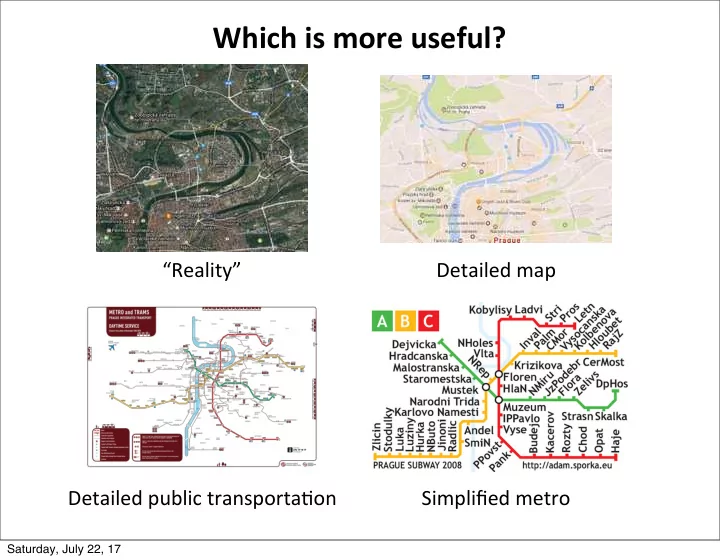
“Reality” Detailed ¡map Detailed ¡public ¡transporta6on Simplified ¡metro
Saturday, July 22, 17
Which is more useful? Reality Detailed map Detailed public - - PowerPoint PPT Presentation
Which is more useful? Reality Detailed map Detailed public transporta6on Simplified metro Saturday, July 22, 17 Models dont need to reflect reality A model is an
“Reality” Detailed ¡map Detailed ¡public ¡transporta6on Simplified ¡metro
Saturday, July 22, 17
designed ¡to ¡eliminate ¡extraneous ¡detail ¡in ¡order ¡to ¡focus ¡ aAen6on ¡on ¡the ¡essen6als ¡of ¡the ¡situa6on. ¡ ¡(Daniel ¡L. ¡Hartl, ¡ 2000)
supply ¡a ¡useful ¡approxima6on ¡to ¡reality: ¡All ¡models ¡are ¡wrong; ¡ some ¡models ¡are ¡useful". ¡ ¡(George ¡E. ¡P. ¡Box, ¡1987)
will ¡not ¡reflect ¡all ¡of ¡reality ¡... ¡While ¡a ¡model ¡can ¡never ¡be ¡ “truth,” ¡a ¡model ¡might ¡be ¡ranked ¡from ¡very ¡useful, ¡to ¡useful, ¡to ¡ somewhat ¡useful ¡to, ¡finally, ¡essen6ally ¡useless. ¡ ¡(Burnham ¡and ¡ Anderson, ¡2002)
model ¡from ¡a ¡predefined ¡set, ¡all ¡of ¡which ¡may ¡be ¡grossly ¡ inadequate ¡as ¡a ¡representa6on ¡of ¡reality. ¡ ¡(J. ¡J. ¡Welch, ¡2006)
Saturday, July 22, 17
Saturday, July 22, 17
(Felsenstein, 1978)
Saturday, July 22, 17
Sequence Length
0.25 0.50 0.75 1.00 2500 5000 7500 10000 Proportion Correct Sequence Length parsimony ML-GTR
Simulation model = GTR
Saturday, July 22, 17
Saturday, July 22, 17
Saturday, July 22, 17
Saturday, July 22, 17
Saturday, July 22, 17
Saturday, July 22, 17
Saturday, July 22, 17
Saturday, July 22, 17
Saturday, July 22, 17
B B B B B B B B
40 80 120 25 50 75 100 y x B B B B B B B B 20 40 60 80 100 25 50 75 100 y x
y =1.30 + 0.965x (r 2 = 0.963) y = - 330 +134x - 15.5x2 +0.816x3
(r 2 =1.000)
Saturday, July 22, 17
Saturday, July 22, 17
Parsimony ¡in ¡sta,s,cs ¡represents ¡a ¡tradeoff ¡between ¡bias ¡and ¡ variance ¡as ¡a ¡func,on ¡of ¡the ¡dimension ¡of ¡the ¡model. ¡ ¡A ¡good ¡ model ¡is ¡a ¡balance ¡between ¡under-‑ ¡and ¡over-‑fi>ng. ¡(Burnham ¡ and ¡Anderson, ¡1998)
Saturday, July 22, 17
Parsimony ¡in ¡sta,s,cs ¡represents ¡a ¡tradeoff ¡between ¡bias ¡and ¡ variance ¡as ¡a ¡func,on ¡of ¡the ¡dimension ¡of ¡the ¡model. ¡ ¡A ¡good ¡ model ¡is ¡a ¡balance ¡between ¡under-‑ ¡and ¡over-‑fi>ng. ¡(Burnham ¡ and ¡Anderson, ¡1998)
Saturday, July 22, 17
Parsimony ¡in ¡sta,s,cs ¡represents ¡a ¡tradeoff ¡between ¡bias ¡and ¡ variance ¡as ¡a ¡func,on ¡of ¡the ¡dimension ¡of ¡the ¡model. ¡ ¡A ¡good ¡ model ¡is ¡a ¡balance ¡between ¡under-‑ ¡and ¡over-‑fi>ng. ¡(Burnham ¡ and ¡Anderson, ¡1998)
B B B B B B B B
40 80 120 25 50 75 100 y x B B B B B B B B 20 40 60 80 100 25 50 75 100 y x
y =1.30 + 0.965x (r 2 = 0.963) y = - 330 +134x - 15.5x2 +0.816x3
(r 2 =1.000)
Saturday, July 22, 17
Assertion: In most situations, phylogenetic inference is relatively robust to model misspecification, as long as critical factors influencing sequence evolution are accommodated Caveat: There are some kinds of model misspecification that are very difficult to overcome (e.g., “heterotachy”) A B C D A B C D Half of sites Other half Likelihood can be consistent in Felsenstein zone, but will be inconsistent if a single set of branch lengths are assumed when there are actually two sets of branch lengths (Chang 1996) (“heterotachy”) E.g.:
Saturday, July 22, 17
GTR SYM TrN F81 JC K3ST K2P HKY85 F84
Equal base frequencies 3 substitution types (transitions, 2 transversion classes) 2 substitution types (transitions vs. transversions) 3 substitution types (transversions, 2 transition classes) 2 substitution types (transitions vs. transversions) Single substitution type Equal base frequencies Single substitution type Equal base frequencies
(general time-reversible) (Tamura-Nei) (Hasegawa-Kishino-Yano) (Felsenstein) Jukes-Cantor (Kimura 2-parameter) (Kimura 3-subst. type) (Felsenstein)
Saturday, July 22, 17
– Some sites extremely unlikely to change due to strong functional or structural constraint (Hasegawa et al., 1985)
– Rate variation assumed to follow a gamma distribution with shape parameter α
– Different relative rates assumed for pre-assigned subsets of sites Lemur AAGCTTCATAG TTGCATCATCCA …TTACATCATCCA Homo AAGCTTCACCG TTGCATCATCCA …TTACATCCTCAT Pan AAGCTTCACCG TTACGCCATCCA …TTACATCCTCAT Goril AAGCTTCACCG TTACGCCATCCA …CCCACGGACTTA Pongo AAGCTTCACCG TTACGCCATCCT …GCAACCACCCTC Hylo AAGCTTTACAG TTACATTATCCG …TGCAACCGTCCT Maca AAGCTTTTCCG TTACATTATCCG …CGCAACCATCCT
Saturday, July 22, 17
…can also include a proportion of “invariable” sites (pinv)
0.02 0.04 0.06 0.08 1 2
Rate
α=50 α=200 α=2 α=0.5
Frequency
Saturday, July 22, 17
Sequence Length
Propo rtion C
Tree
α = 0.5, pinv=0.5 α = 1.0, pinv=0.5 α = 1.0, pinv=0.2
0.1 0.2 0.3 0.4 0.5 0.6 0.7 0.8 0.9 1 100 1000 1000 10000 GTRi g GTRg HKYg GTRi HKYi GTRer HKYer parsimony HKYi g GTRi g GTRg HKYg GTRi HKYi GTRer HKYer parsimony HKYi g 0.1 0.2 0.3 0.4 0.5 0.6 0.7 0.8 0.9 1 100 1000 1000 10000 GTRi g GTRg HKYg GTRi HKYi GTRer HKYer parsimony HKYi g 0.1 0.2 0.3 0.4 0.5 0.6 0.7 0.8 0.9 1 100 1000 1000 10000 0.1 0.2 0.3 0.4 0.5 0.6 0.7 0.8 0.9 1 100 1000 1000 10000 GTRi g HKYi g GTRg HKYg GTRi HKYi GTRer HKYer Parsimony 0.1 0.2 0.3 0.4 0.5 0.6 0.7 0.8 0.9 1 100 1000 1000 10000 GTRi g HKYi g GTRg HKT g GTRi HKYi GTRer HKYer parsimony 0.1 0.2 0.3 0.4 0.5 0.6 0.7 0.8 0.9 1 100 1000 1000 10000 GTRig HYYig GTRg HKYg GTRi HKYi GRTer HKYer parsimony 0.1 0.2 0.3 0.4 0.5 0.6 0.7 0.8 0.9 1 100 1000 1000 10000 GTRig GTRg HKYg GTRi HKYi GTRer HKYer parsimony HKYi g 0.1 0.2 0.3 0.4 0.5 0.6 0.7 0.8 0.9 1 100 1000 1000 10000 GTRi g GTRg HKYg GTRi HKYi GTRer HKYer parsimony HKYi g 0.1 0.2 0.3 0.4 0.5 0.6 0.7 0.8 0.9 1 100 1000 1000 10000Saturday, July 22, 17
0.1 0.2 0.3 0.4 0.5 0.6 0.7 0.8 0.9 1 100 1000 10000 100000 JCer JC+G JC+I JC+I+G GTRer GTR+G GTR+I GTR+I+G parsimon y
Saturday, July 22, 17
0.1 0.2 0.3 0.4 0.5 0.6 0.7 0.8 0.9 1 100 1000 10000 100000 JCer JC+G JC+I JC+I+G GTRer GTR+G GTR+I GTR+I+G parsimon y
Saturday, July 22, 17
δ = −2 ln L0 − ln L1
If model L0 is nested within model L1, δ is distributed as X2 with degrees-of-freedom equal to difference in number of free parameters
Saturday, July 22, 17
Histogram of δ = −2 ln L0 − ln L1
JC vs K80 models
Saturday, July 22, 17
X2 3.84 6.64 0.05 and 0.01 critical values
Histogram of δ = −2 ln L0 − ln L1
JC vs K80 models
Saturday, July 22, 17
Saturday, July 22, 17
Saturday, July 22, 17
AICi = −2lnLi + 2K
where K is the number of free parameters estimated
Saturday, July 22, 17
AICi = −2lnLi + 2K
where K is the number of free parameters estimated
Saturday, July 22, 17
AICi = −2lnLi + 2K
where K is the number of free parameters estimated
Saturday, July 22, 17
AICi = −2lnLi + 2K
where K is the number of free parameters estimated
BICi = −2lnLi + K lnn
where K is the number of free parameters estimated and n is the “sample size” (typically number of sites)
Saturday, July 22, 17
– BIC performs well when true model is contained in model set, and among a set of simple models, AIC often selects a more complex model than the truth (indeed, AIC is formally statistically inconsistent) – But in phylogenetics, no model is as complex as the truth, and the true model will never be contained in the model set. – BIC often chooses models that seem too simple, however.
Saturday, July 22, 17
Saturday, July 22, 17
Yang ¡and ¡Rannala ¡(2012; ¡Nature ¡Rev. ¡Genet. ¡13:303-‑314)
Saturday, July 22, 17
e.g., ¡Simon ¡et ¡al., ¡2006)
Saturday, July 22, 17
Saturday, July 22, 17
Saturday, July 22, 17
1.2, ¡0.9, ¡1.1, ¡0.95)
Saturday, July 22, 17
1.2, ¡0.9, ¡1.1, ¡0.95)
These ¡are ¡all ¡GTR ¡models ¡that ¡are ¡not ¡far ¡from ¡the ¡ Jukes-‑Cantor ¡model, ¡but ¡they ¡all ¡have ¡different ¡ names
BeAer ¡to ¡es6mate ¡one ¡GTR ¡model ¡(even ¡with ¡5+3+1+1=10 ¡parameters, ¡ es6mated ¡from ¡all ¡data) ¡than ¡3 ¡separate ¡models ¡with ¡2+5+1=8 ¡parameters ¡ (but ¡only ¡one ¡gene’s ¡worth ¡of ¡data ¡for ¡each ¡model)
Saturday, July 22, 17
Rob ¡Lanfear’s ¡Par88onFinder ¡(hAp://www.robertlanfear.com/par66onfinder/) ¡ automates ¡this ¡process; ¡method ¡now ¡also ¡available ¡in ¡PAUP* ¡test ¡versions
Saturday, July 22, 17
N Bell number 2 3 4 5 6 7 12 60 2 5 52 203 877 4140 4 x 10⁶ 9.8 x 1059
Saturday, July 22, 17
Lanfear, R., Calcott, B., Ho, S. Y. W., & Guindon, S. (2012). Partitionfinder: combined selection of partitioning schemes and substitution models for phylogenetic analyses. Molecular Biology and Evolution, 29(6), 1695– 1701
Saturday, July 22, 17
Lanfear, R., Calcott, B., Ho, S. Y. W., & Guindon, S. (2012). Partitionfinder: combined selection of partitioning schemes and substitution models for phylogenetic analyses. Molecular Biology and Evolution, 29(6), 1695– 1701
Saturday, July 22, 17
Lanfear, R., Calcott, B., Ho, S. Y. W., & Guindon, S. (2012). Partitionfinder: combined selection of partitioning schemes and substitution models for phylogenetic analyses. Molecular Biology and Evolution, 29(6), 1695– 1701
Saturday, July 22, 17
Lanfear, R., Calcott, B., Ho, S. Y. W., & Guindon, S. (2012). Partitionfinder: combined selection of partitioning schemes and substitution models for phylogenetic analyses. Molecular Biology and Evolution, 29(6), 1695– 1701
Saturday, July 22, 17
Lanfear, R., Calcott, B., Ho, S. Y. W., & Guindon, S. (2012). Partitionfinder: combined selection of partitioning schemes and substitution models for phylogenetic analyses. Molecular Biology and Evolution, 29(6), 1695– 1701
Saturday, July 22, 17
Lanfear, R., Calcott, B., Ho, S. Y. W., & Guindon, S. (2012). Partitionfinder: combined selection of partitioning schemes and substitution models for phylogenetic analyses. Molecular Biology and Evolution, 29(6), 1695– 1701
Saturday, July 22, 17
Lanfear, R., Calcott, B., Ho, S. Y. W., & Guindon, S. (2012). Partitionfinder: combined selection of partitioning schemes and substitution models for phylogenetic analyses. Molecular Biology and Evolution, 29(6), 1695– 1701
Saturday, July 22, 17
Lanfear, R., Calcott, B., Ho, S. Y. W., & Guindon, S. (2012). Partitionfinder: combined selection of partitioning schemes and substitution models for phylogenetic analyses. Molecular Biology and Evolution, 29(6), 1695– 1701
Saturday, July 22, 17
Lanfear, R., Calcott, B., Ho, S. Y. W., & Guindon, S. (2012). Partitionfinder: combined selection of partitioning schemes and substitution models for phylogenetic analyses. Molecular Biology and Evolution, 29(6), 1695– 1701
Saturday, July 22, 17
Lanfear, R., Calcott, B., Ho, S. Y. W., & Guindon, S. (2012). Partitionfinder: combined selection of partitioning schemes and substitution models for phylogenetic analyses. Molecular Biology and Evolution, 29(6), 1695– 1701
Saturday, July 22, 17
Lanfear, R., Calcott, B., Ho, S. Y. W., & Guindon, S. (2012). Partitionfinder: combined selection of partitioning schemes and substitution models for phylogenetic analyses. Molecular Biology and Evolution, 29(6), 1695– 1701
Saturday, July 22, 17
Lanfear, R., Calcott, B., Ho, S. Y. W., & Guindon, S. (2012). Partitionfinder: combined selection of partitioning schemes and substitution models for phylogenetic analyses. Molecular Biology and Evolution, 29(6), 1695– 1701
Saturday, July 22, 17
Lanfear, R., Calcott, B., Ho, S. Y. W., & Guindon, S. (2012). Partitionfinder: combined selection of partitioning schemes and substitution models for phylogenetic analyses. Molecular Biology and Evolution, 29(6), 1695– 1701
Saturday, July 22, 17
1 ¡+ ¡n(n2 ¡-‑ ¡1)/6 ¡= ¡11 ¡schemes
For ¡1265 ¡genes, ¡there ¡would ¡s,ll ¡be ¡ 337,380,561 ¡schemes ¡to ¡evaluate!
Lanfear, R., Calcott, B., Ho, S. Y. W., & Guindon, S. (2012). Partitionfinder: combined selection of partitioning schemes and substitution models for phylogenetic analyses. Molecular Biology and Evolution, 29(6), 1695– 1701
Saturday, July 22, 17
Saturday, July 22, 17
Es6mate ¡model ¡parameters ¡on ¡a ¡shared ¡model; ¡similar ¡subsets ¡ will ¡have ¡similar ¡parameter ¡es6mates ¡and ¡will ¡cluster ¡together.
Problem? ¡ ¡Similar ¡models ¡(in ¡the ¡sense ¡of ¡predic,ng ¡similar ¡site ¡paSern ¡ frequencies), ¡can ¡have ¡different ¡parameter ¡MLEs. ¡ ¡Must ¡use ¡same ¡model ¡ for ¡all ¡subsets.
Hierarchical ¡(or ¡non-‑hierarchical ¡kmeans) ¡clustering ¡using ¡ same ¡idea ¡as ¡Li ¡et ¡al. ¡(very ¡efficient ¡implementa6on)
Saturday, July 22, 17