Very Slow Diffusion Processes and its Regional Analysis ICERM FPDE - - PowerPoint PPT Presentation

FUGITIVE METHANE DETECTION AND LOCALIZATION WITH SMALL UNMANNED AERIAL SYSTEMS: CHALLENGES AND OPPORTUNITIES

DEREK HOLLENBECK, YANGQUAN CHEN Department of Mechanical Engineering, University of California, Merced.

Contact: {dhollenbeck,ychen53}@ucmerced.edu Acknowledgements: NSF NRT Fellowship (http://www.nrt-ias.org)

REFERENCES

[1] Matheou et al. Environ Fluid Mech., 2016. [2] Li et al. Int. Conf. on Rob. and Biomim., 2009. [3] Smith et al. ICUAS Miami., 2017. [4] Farrell et al. Env. Fluid Mech., 2002. [5] Nurzaman et al. PLos ONE, 2011.

INTRODUCTION

Natural gas is one of our main methods to gener- ate power today. Utility companies that provide this gas are tasked with maintaining and survey- ing leaks. These leaks are referred to as fugitive methane emissions and detecting these fugitive gases can be pivotal to preventing incidents such as the San Bruno explosion, killing 8 and injur- ing dozens due to a gas leak going undetected. Recently, using NASA technology onboard low cost vertical takeoff and landing (VTOL) small unmanned aerial systems (sUAS) we can detect fugitive methane at 1 ppb (parts per billion) lev- els.

CHALLENGES IN DETECTION

General challenges include: FAA regulations (no flights over people), battery life, and complex dy- namic plume behavior. Factors that impact de- tection can be: propeller wash, sensor placement, wind, and mechanical/electrical noises. Even distance to source and flight altitudes can change the probability of detection (Sigmoid like) scal- ing with topology and atmospheric stability. Lo- calization by CFD approaches are costly making real-time estimations and visualizations difficult.

QUASI-STEADY INVERSION

Following the work by Matthes et al (2005), Carslaw (1959), and Roberts (1923) the solution to a single point source advection diffusion equa- tion (ADE) can be solved for a dynamic system approximately by making a quasi-steady state as- sumption if the variance and transient behavior

• f the wind small. W0 is the Lambert function.

∂C ∂t − D∂2C ∂x2

i

+ v ∂C ∂xi = 2q0δ(t − t0)δ(xi − xi0) ¯ C(¯ xi, x0, qo)i = q0 exp( ¯

v(¯ xi−x0) 2D

) π

2 3 Dd

di(Ci, x0, q0) ≈ 2D ¯ v W0( ¯ vq0 4πD2Ci exp( v 2D(¯ xi−x0))) min

q0,x0 : m

• i,j=1

(y0,i(x0, q0) − y0,j(x0, q0))2

ADAPTIVE SEARCH MODEL

In the foraging literature the Levy walk has been shown to be effective at searching sparse environ-

• ments. However, Brownian motion is more effi-

cient in dense areas. This adaptive search model [5] can switch dynamically from Levy to Brown- ian based on finding targets using tumble proba- bility P(x(t)), x(t) is governed by the stochastic differential equation (SDE) below P(x(t)) = e−x(t), 0 ≤ x ≤ 5 ˙ x = −∂U ∂x A+ǫ,      U = (x − h)2, ǫ :

• H = 1

2, N(0, σ)

H = 1

2, fGn

A = max(Amin, α(t)) αk = Cααk−1 + ktF

• F = 1, found target

F = 0, otherwise. we extend [5] by adding, fGn, defined as Yj = BH(j + 1) − BH(j) and fraction Brownian motion is given below.

ADAPTIVE SEARCH AND LOCALIZATION

The adaptive search model has shown to adjust from Brownian motion to Levy walks in a 2D ran- dom search. By reducing the problem to a 1D path problem (i.e. survey route) adding decision trees and modeling fugitive gas with a small time scale filament model [4] we have the opportunity to optimize random search for application. Gather enough information to form a sample(s) to use in the inversion method for a Zeroth order approxi- mation of source localization (x0,y0) and quantifi- cation (q0). BH(x) ≈

• φ(x − y)B(∆y)

φ(x) = Γ(H + 1 − d/2 + ||x||) Γ(||x|| + 1)Γ(H + 1 − d/2) ≈ ||x||H−d/2 Γ(H + 1 − d/2)

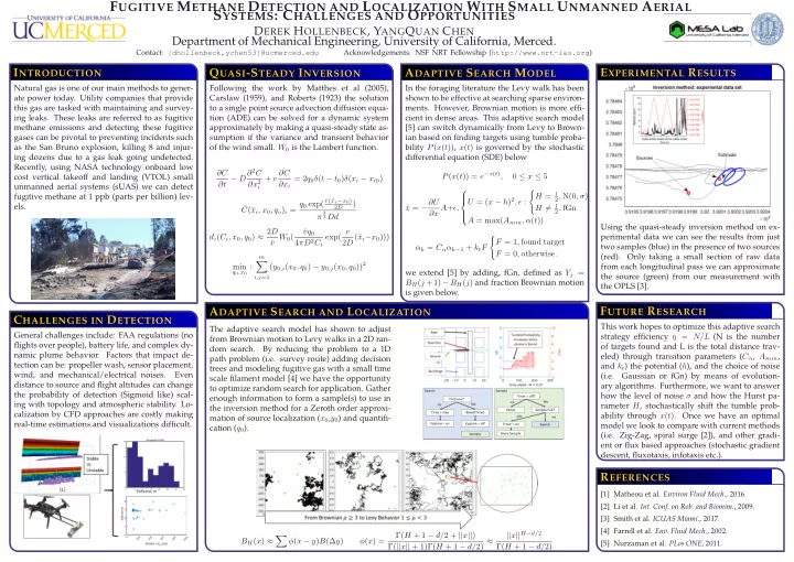
EXPERIMENTAL RESULTS

Using the quasi-steady inversion method on ex- perimental data we can see the results from just two samples (blue) in the presence of two sources (red). Only taking a small section of raw data from each longitudinal pass we can approximate the source (green) from our measurement with the OPLS [3].

FUTURE RESEARCH

This work hopes to optimize this adaptive search strategy efficiency η = N/L (N is the number

• f targets found and L is the total distance trav-

eled) through transition parameters (Cα, Amin, and kt) the potential (h), and the choice of noise (i.e. Gaussian or fGn) by means of evolution- ary algorithms. Furthermore, we want to answer how the level of noise σ and how the Hurst pa- rameter H, stochastically shift the tumble prob- ability through x(t). Once we have an optimal model we look to compare with current methods (i.e. Zig-Zag, spiral surge [2]), and other gradi- ent or flux based approaches (stochastic gradient descent, fluxotaxis, infotaxis etc.).

Very Slow Diffusion Processes and its Regional Analysis

ICERM FPDE Workshop 2018, Brown University Presenter: Dr. YangQuan Chen The MESA Lab, University of California, Merced Joint work with Ruiyang Cai (Donghua University, China) and Yuquan Chen (University of Science and Technology of China) June 21, 2018 June 21, 2018

Main Contents

• 1. Very Slow Tail

Background Comparison with other tails Laplace transform of the very slow kernel

• 2. New Fractional Integral and Derivative

Definitions Integral and derivative of some special functions Realization of L−1

log s sα(s−1)

• (t) by NILT and Prony
• 3. Regional Analysis

Introduction to the regional analysis Regional observability and controllability

• 4. Further Research Directions
• 5. Main References

Background

Figure: Tesla Model S/X Mileage VS Remaining Battery Capacity

Background

Figure: Tesla Model S/X Battery Age VS Remaining Battery Capacity

Some Links

https://docs.google.com/spreadsheets/d/t024 bMoRiDPIDialGnuKPsg/edit#gid=1669966328 https://docs.google.com/spreadsheets/d/t024 bMoRiDPIDialGnuKPsg/edit#gid=154312675 For more details, see [1].

Background

Figure: Human feet as a geological force

https://twitter.com/PaulMMCooper/status/1007612133356572672

Different tails to describe decay rate

For the above data, t−α is too fast while (log t)−α is too slow

Very Slow between power-law and ultra-slow? Yes!

A new tail for very-slow: log t

tα

Image of these kernels: x label-t

500 1000 0.5 1 1.5

α=0.25

500 1000 0.2 0.4 0.6 0.8

α=0.5

500 1000 0.2 0.4 0.6

α=0.75

500 1000 0.2 0.4 0.6

α=1

exp(-t)/tα log(t)/tα 1/tα 1/(log(t))α () June 21, 2018 8 / 43

Image of these kernels: x label-log t

2 4 6 8 0.5 1 1.5

α=0.25

2 4 6 8 0.2 0.4 0.6 0.8

α=0.5

2 4 6 8 0.2 0.4 0.6

α=0.75

2 4 6 8 0.2 0.4 0.6

α=1

exp(-t)/tα log(t)/tα 1/tα 1/(log(t))α () June 21, 2018 9 / 43

Comparison between log t

tα and 1 (log t)α when α = 0.25

0.5 1 1.5 2 2.5 3 3.5 4 4.5 5 ×106 0.5 1 1.5

x-lable: t

log(t)/tα 1/(log(t))α

101 102 103 104 105 106 107 0.5 1 1.5

x-lable: log t

log(t)/tα 1/(log(t))α () June 21, 2018 10 / 43

Laplace transform of the very slow kernel

The Laplace transform of the very slow kernel is L log t tα

• (s) = sα−1Γ(1 − α) (ψ(1 − α) − log s) ,

where ψ(x) = Γ′(x)

Γ(x) denotes the digamma function.

Realization of the kernel in engineering by Prony

• 50
• 40
• 30
• 20
• 10

Figure: Prony: α=0.5, order=12, t=10, Ts=0.01

Realization of the kernel in engineering by Prony

• 20

• 200
• 100

Figure: Bode diagram: α=0.5, order=12

Realization of the kernel in engineering by Prony

• 1
• 0.5

• 1
• 0.8
• 0.6
• 0.4
• 0.2

Figure: Pole-Zero: α=0.5, order=12

Definitions

α-th order fractional integral:

0I α t f (t)

1 Γ(α) t log(t − s) (t − s)1−α f (s)ds α-th order Riemann-Liouville type fractional derivative:

0Dα t f (t)

1 Γ(1 − α) d dt t log(t − s) (t − s)α f (s)ds α-th order Caputo type fractional derivative:

C 0 Dα t f (t)

1 Γ(1 − α) t log(t − s) (t − s)α f ′(s)ds

Properties

Dαf (t) = d

dt I 1−αf (t) 0I β t 0I α t f (t) =0 I α t 0I β t f (t) =0 I α+β t

f (t)

0Dβ t 0Dα t f (t) =0 Dα t 0Dβ t f (t) =0 Dα+β t

f (t)

C 0 Dβ t C 0 Dα t f (t) =C 0 Dα t C 0 Dβ t f (t) =C 0 Dα+β t

f (t)

Integral and derivative of some special functions

f (t) = 1:

0I α t 1 = tα Γ(α+1)

• log t − 1

α

• 0Dα

t 1 = 1 Γ(1−α)t−α log t C 0 Dα t 1 = 0

Integral and derivative of some special functions

f (t) = tk:

0I α t tk = Γ(k+1) Γ(k+α+1)tk+α (log t + ψ(α) − ψ(k + α + 1)) 0Dα t tk =

• Γ(k+1)

Γ(k−α+2) + Γ(k+1) Γ(k−α+1) (ψ(1 − α) − ψ(k − α + 2))

• tk−α

+

Γ(k+1) Γ(k−α+1)tk−α log t C 0 Dα t tk = Γ(k+1) Γ(k−α+1)tk−α (log t + ψ(1 − α) − ψ(k − α + 1))

Integral and derivative of some special functions

f (t) = exp(t):

0I α t exp(t) = ψ(α)(Γ(α)−Γ(α,t)) Γ(α)

exp(t) − L−1

log s sα(s−1)

• (t)

0Dα t exp(t) =C 0 Dα t exp(t) = d dt

• 0I 1−α

t

exp(t)

• where Γ(α, t) is the upper incomplete Gamma function defined by

Γ(α, t) = ∞

t

xα−1 exp(−x)dx

Realization of L−1

log s sα(s−1)

• (t) by NILT and Prony

Figure: NILT: α=0.4, order=3, t=10, Ts=0.001

G(z−1) = 0.9942z2 − 1.988z + 0.9936 z3 − 2.999z2 + 2.998z − 0.9992

Realization of L−1

log s sα(s−1)

• (t) by NILT and Prony

• 50

• 120
• 100
• 80
• 60
• 40

Figure: Bode diagram: α=0.4, order=3, Ss=0.01

Realization of L−1

log s sα(s−1)

• (t) by NILT and Prony

Figure: NILT: α=0.4, order=5, t=100, Ts=0.01

G(z−1) = 0.9942z4 − 3.904z3 + 5.749z2 − 3.761z + 0.9225 z5 − 4.925z4 + 9.703z3 − 9.555z2 + 4.705z − 0.9264

Realization of L−1

log s sα(s−1)

• (t) by NILT and Prony

• 50

• 120
• 100
• 80
• 60
• 40

Figure: Bode diagram: α=0.4, order=5, Ss=0.01

MATLAB NILT toolbox: https://www.mathworks.com/matlabcentral/fileexchange/39035- numerical-inverse-laplace-transform?s tid=srchtitle More theory and applications of NILT, see [2] MATLAB Prony toolbox: see [3]

What is regional analysis

In 1988, El Jai et al. first introduced the ”regional analysis” [4]. Briefly speaking, regional analysis is to control, observe, stabilize or detect the considered systems on a sub-region of the whole domain of interest.

Our works on the regional analysis of fractional order PDEs

Sub-diffusion Controllability (normal, gradient, boundary; exact, approximate) Observability (normal, gradient, boundary; exact, approximate) Detection of unknown sources Spreadability Stability and stabilizability (normal, boundary) Ultra-slow diffusion Controllability (normal, gradient; exact, approximate) Observability (normal, gradient; exact, approximate)

Main works

Ge F, Chen YQ, Kou C, Podlubny I.Fractional Calculus and Applied Analysis, 2016. Ge F, Chen YQ, Kou C. Journal of Mathematical Analysis and Applications, 2016. Ge F, Chen YQ, Kou C. Automatica, 2016. Ge F, Chen YQ, Kou C. Journal of Mathematical Analysis and Applications, 2016. Ge F, Chen YQ, Kou C. Automatica, 2017. Ge F, Chen YQ, Kou C. IMA Journal of Mathematical Control and Information, 2017. Ge F, Chen YQ, Kou C. Springer, 2018 [5]. The first monograph about the regional analysis of fractional diffusion processes.

Motivation

Figure: Monitoring the fire and managing to put it out

How many sensors (UAVs) and actuators (fire extinguishers)?

Why we need regional analysis

More efficient Reduction in the number of actuators and sensors Reduce the computational requirements Discuss the systems which are not controllable/observable/stable/ detectable on the whole domain

Problem statement

Consider the following time fractional order diffusion system with the Caputo type of our new time fractional derivative:     

C a Dα t y(x, t) = Ay(x, t) + Bu(t) in Υ,

y(x, a) = y0(x) in Ω, y(ξ, t) = 0 on Σ, (1) where Υ = Ω × [a, b], Σ = ∂Ω × [a, b] and 0 < α < 1. A is an infinitesimal generator of a C0−semigroup {T(t)} on the Hilbert space L2(Ω), while −A a uniformly elliptic operator. The initial vector y0 ∈ L2(Ω) is unknown in observability problem. u(t) ∈ Rm, B : Rm → L2(Ω) is a bounded linear operator.

Problem statement

The measurements are given by the output function: z(x, t) = Cy(x, t), (2) where C: L2 (Ω × [a, b]) → L2 (a, b; Rm) is a bounded operator with dense domain, m donates the number of sensors.

How to use the regional analysis

The considered system is said to be regional exactly controllable on ω at time b, if for every yb ∈ L2(ω), there exists a u ∈ L2 ([a, b], Rm) such that pωyu(x, b) = yb, where pω is the restriction map from Ω to its subset ω. The considered system is said to be regionally exactly observable in ω, if pωy0 ⊆ L2(Ω) can be uniquely determined by z(x, t).

Methods

DPSs(distributed parameter systems): the state depends on the spatial distribution and the state space is infinite-dimensional. Typical examples: systems described partial differential equations, integral equations and functional differential equations. Properties of the partial differential equations(PDEs) Theory of infinite-dimensional linear systems Semigroups and functional analysis Lie algebra

When we need regional analysis

Complex systems Need plenty of actuators and sensors Difficulty in computation Discuss the systems which are not controllable/observable/stable/ detectable on the whole domain

Solution of system (1)-(2)

For observability problem, Bu(t) = 0 in (1). Applying Laplace transform and its inverse on (1), we obtain y(x, t) = G(t)y0(x), where G(t) = L−1 sα−1 (ψ(1 − α) − log s) · (sα (ψ(1 − α) − log s) I − A)−1 (t). And z(x, t) = CG(t)y0(x).

Theoretical results

Denote Q = CG, H = pωQ∗, where Q∗ is the adjoint operator of Q. Then we have the following equivalent conditions. System (1)-(2) is regionally exactly observable in ω; Im (H) = L2(ω); Ker (pω) + Im(Q∗) = L2(Ω); There is a constant c > 0 such that, z ∈ L2(ω), zL2(ω) ≤ c H∗zL2(a,b;Rm) . We can also obtain some similar equivalent conditions for regional approximate observability.

Minimum number of sensors

For zone sensors, zi(t) =

• Pi di(x)y(x, t)dx, where Pi ⊆ Ω stands for

the location of the i-th sensor and di is its corresponding spatial distribution, i = 1, . . . , m. Let rk be the multiplicities of the k-th eigenvalue λk of A, αkj(x) be the j-th eigenfunction of λk. Denote χPi be the indicator function on Pi, di

kj(x) = χPidi(x), αkj(x) and define

Dk =    d1

k1(x)

· · · d1

krk(x)

. . . · · · . . . dm

k1(x)

· · · dm

krk(x)

   . Then the sensors (Pi, di(x)) , i = 1, . . . , m are ω−strategic if and only if m ≥ r sup {rk} and rank Dk = rk, for k = 1, 2, . . . .

Solution of system (1)

For controllability problem, y(x, t) = G(t)y0(x) + G(t), where

• G(t) = L−1

(sα (ψ(1 − α) − log s) I − A)−1 F(s)

• (t).

Here, F(s) is the Laplace transform of Bu(t).

Theoretical results

Define Hu = yu(x, b), then the following conditions are equivalent: System (1)-(2) is regionally exactly controllable in ω; Im

• pω

H

• = L2(ω);

Ker (pω) + Im( H) = L2(Ω); There is a constant c > 0 such that, y ∈ L2(ω), yL2(ω) ≤ c

• H∗p∗

ωy

• L2(a,b;Rm) .

We can also obtain some similar equivalent conditions for regional approximate controllability.

Minimum number of sensors

For zone sensors, Bu = m

i=1 χPidi(x)ui(t). Define

Dk =    d1

k1(x)

· · · d1

krk(x)

. . . · · · . . . dm

k1(x)

· · · dm

krk(x)

   . Then the actuators (Pi, di(x)) , i = 1, . . . , m are ω−strategic if and only if m ≥ r sup {rk} and rank Dk = rk, for k = 1, 2, . . . .

Further Research Directions

Optimal sensors/actuators placements Regional gradient observability/controllability Mobile sensors/actuators Semi-linear or nonlinear systems Stochastic PDEs

Main references

1 Steinbuch M. Tesla Model S battery degradation data[DB/OL]. https://steinbuch.wordpress.com/2015/01/24/tesla-model-s-battery- degradation-data/,2015-01-24/2018-06-12. 2 Sheng H, Li Y, Chen YQ. Application of numerical inverse Laplace transform algorithms in fractional calculus[J]. Journal of the Franklin Institute, 2011, 348(2):315-330. 3 https://www.mathworks.com/matlabcentral/fileexchange/3955- prony-toolbox 4 Jai AE, Pritchard AJ. Sensors and Controls in the Analysis of Distributed Systems[M]. Halsted Press, 1988. 5 Ge F, Chen YQ, Kou C. Regional Analysis of Time-Fractional Diffusion Processes[M]. Springer, 2018.

Thanks for your attention! Questions?