31/10/2019 Diffusion General Note. Atomic diffusion is a process - - PowerPoint PPT Presentation

SLIDE 1

31/10/2019 1

Diffusion

Factors that Influence Diffusion

 Temperature - diffusion rate increases very rapidly with increasing temperature  Diffusion mechanism - interstitial is usually faster than vacancy  Diffusing and host species - Do, Qd is different for every solute, solvent pair  Microstructure - diffusion faster in polycrystalline vs. single crystal materials because of the rapid diffusion along grain boundaries and dislocation cores. Atomic diffusion is a process whereby the random thermally-activated hopping of atoms in a solid results in the net transport of atoms. For example, helium atoms inside a balloon can diffuse through the wall of the balloon and escape, resulting in the balloon slowly deflating. Other air molecules (e.g. oxygen, nitrogen) have lower mobilities and thus diffuse more slowly through the balloon wall. There is a concentration gradient in the balloon wall, because the balloon was initially filled with helium, and thus there is plenty of helium on the inside, but there is relatively little helium on the outside (helium is not a major component of air).

1

General Note. Diffusion is a flux of matter in which the atoms or molecules of a certain type move differently (rate, amount etc) with respect to the atoms/molecules of other type.  Please note the difference from gas or liquid flow, in this case ALL components move in the same way.  The definition: “Diffusion is the movement of molecules from a high concentration to a low concentration” is wrong because there are cases when diffusion process does just opposite.  Flux of matter can be caused not only by the difference in concentration of the atom that diffuses, but also the difference in concentration of other atoms and or gradient of physical parameters ( temperature, pressure, electric or magnetic field).

2

Diffusion

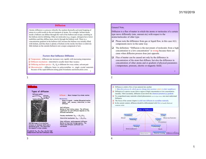
Types of diffusion

Diffusion paths: HRTEM image of an interface between an aluminum (left) and a germanium grain. The black dots correspond to atom columns.

Surface diffusion Bulk diffusion Grain baoundary diffusion

In general: Dgp >Dsd >Dgb >>Db for high temperatures and short diffusion times

Diffusion through the gas phase

Self diffusion: Motion of host lattice atoms. The diffusion coefficient for self diffusion depends on the diffusion mechanism: Vacancy mechanism: Dself = [Cvac] Dvac Interstitial mechanism: Dself = [Cint] Dint Inter diffusion, multicomponent diffusion: Motion of host and foreign species. The fluxes and diffusion coefficient are correlated Diffusion - Mass transport by atomic motion Mechanisms

• Gases & Liquids – random (Brownian) motion
• Solids – self, vacancy, interstitial, or inter

diffusion 3

Oxidation

Roles of Diffusion

Creep Aging Sintering Doping Carburizing Metals Precipitates Steels Semiconductors Many more… Many mechanisms Material Joining Diffusion bonding  Diffusion is relative flow of one material into another

• Mass flow process by which species change their position relative to their neighbours.

 Diffusion of a species occurs from a region of high concentration to low concentration (usually). More accurately, diffusion occurs down the chemical potential (µ) gradient.  To comprehend many materials related phenomenon (as in the figure below) one must understand Diffusion.  The focus of the current chapter is solid state diffusion in crystalline materials.  In the current context, diffusion should be differentiated with flow (of usually fluids and

sometime solids). 4

1 2 3 4

SLIDE 2

31/10/2019 2

Processing Using Diffusion

 Case Hardening:

• Diffuse carbon atoms into

the host iron atoms at the surface.

• Example of interstitial

diffusion is a case hardened gear.

 Result: The presence of C atoms makes iron (steel) harder.

• Doping silicon with phosphorus for n-type

semiconductors:

• Process:
• 3. Result: Doped

semiconductor regions. silicon

magnified image of a computer chip

0.5 mm

light regions: Si atoms light regions: Al atoms

• 2. Heat it.
• 1. Deposit P rich

layers on surface. silicon

5

Ar H2

Movable piston with an orifice H2 diffusion direction Ar diffusion direction

Piston motion

Piston moves in the direction of the slower moving species  When a perfume bottle is opened at one end of a room, its smell reaches the other end via the diffusion of the molecules of the perfume.  If we consider an experimental setup as below (with Ar and H2 on different sides of a chamber separated by a movable piston), H2 will diffuse faster towards the left (as compared to Ar). As obvious, this will lead to the motion of movable piston in the direction

• f the slower moving species.

6

A B

Inert Marker is basically a thin rod of a high melting material, which is insoluble in A & B

Kirkendall effect

• Let us consider two materials A and B welded together with Inert marker and given

a diffusion anneal (i.e. heated for diffusion to take place).

• Usually the lower melting component diffuses faster (say B). This will lead to the

shift in the marker position to the right.

Direction of marker motion

7

 Mass flow process by which species change their position relative to their neighbours.  Diffusion is driven by thermal energy and a ‘gradient’ (usually in chemical potential). Gradients in other physical quantities can also lead to diffusion (as in the figure below). In this chapter we will essentially restrict ourselves to concentration gradients.  Usually, concentration gradients imply chemical potential gradients; but there are exceptions to this rule. Hence, sometimes diffusion occurs ‘uphill’ in concentration gradients, but downhill in chemical potential gradients.  Thermal energy leads to thermal vibrations of atoms, leading to atomic jumps.  In the absence of a gradient, atoms will still randomly ‘jump about’, without any net flow of matter.

Diffusion

Chemical potential Electric Gradient Magnetic Stress

• First we will consider a continuum picture of diffusion

and later consider the atomic basis for the same in crystalline solids. The continuum picture is applicable to heat transfer (i.e., is closely related to mathematical equations of heat transfer).

8

5 6 7 8

SLIDE 3

31/10/2019 3

9

 Diffusion mechanisms

• Vacancy diffusion
• Interstitial diffusion
• Impurities

 Conditions necessary for diffusion

• An empty adjacent site
• Enough energy to break bonds and cause lattice distortions during

displacement  Mathematics of diffusion

• Steady-state diffusion (Fick’s first law)
• Nonsteady-State Diffusion (Fick’s second law)

 Factors that influence diffusion

• Diffusing species
• Host solid
• Temperature
• Microstructure

Diffusion – How atoms move in solids

10

What is diffusion?

Diffusion transport by atomic motion.

Inhomogeneous material can become homogeneous by diffusion. Temperature should be high enough to overcome energy barrier.

Diffusion

• Part1. Constitutional effects

Diffusion is the phenomenon of spontaneous material transport by atomic motion. Diffusion is classified according to a) conditions: self-diffusion, diffusion from surface, interdiffusion, fast path diffusion etc. b) mechanism: interstitial, substitutional; Part 2. Non-constitutional effects. Kirkendall effect, Einstein equation, etc.11

12

Atom migration Vacancy migration After Before

Diffusion Mechanisms

Vacancy diffusion  To jump from lattice site to lattice site, atoms need energy to break bonds with neighbors, and to cause the necessary lattice distortions during jump.  Therefore, there is an energy barrier.  Energy comes from thermal energy of atomic vibrations

(Eav ~ kT)

 Atom flow is opposite to vacancy flow direction.

9 10 11 12

SLIDE 4

31/10/2019 4

13

Interstitial atom before diffusion

Interstitial atom after diffusion

Diffusion Mechanisms

Interstitial diffusion  Generally faster than vacancy diffusion because bonding of interstitials to surrounding atoms is normally weaker and there are more interstitial sites than vacancy sites to jump to.  Smaller energy barrier  Only small impurity atoms (e.g. C, H, O) fit into interstitial sites.  The rate of interstitial diffusion is controlled only by the easiness with which a diffusing atom can move into an interstice.

14

Self-diffusion: In an elemental solid, atoms also migrate.

A B C D

After some time

A B C D

Vacancy Diffusion:

• atoms exchange with vacancies
• applies to substitutional impurities atoms
• rate depends on:
• - number of vacancies
• - activation energy to exchange.

increasing elapsed time

Probability of an atom jumping over the energy barrier: 𝑄 = 𝑓𝑦𝑞 − 𝑅 𝑙𝑈

15

Interstitial diffusion – smaller atoms can diffuse between atoms. Interdiffusion: : In an alloy, atoms tend to migrate from regions of high conc. to regions of low conc.

More rapid than vacancy diffusion

Initially After some time There is an energy barrier which must be overcome when an atom changes site.

Mechanisms of interdiffusion:

16

13 14 15 16

SLIDE 5

31/10/2019 5

17

Before After (Heat)

Inter-diffusion vs. Self-diffusion

Self-diffusion: One-component material, atoms are of same type.

1 dn J A dt 

Flow direction Area (A)  Concentration gradient. Concentration can be designated in many ways (e.g. moles per unit volume). Concentration gradient is the difference in concentration between two points (usually close by).  We can use a restricted definition of flux (J) as flow per unit area per unit time: → mass flow / area / time  [Atoms / m2 / s].  Steady state. The properties at a single point in the system does not change with time. These properties in the case of fluid flow are pressure, temperature, velocity and mass flow rate.

• In the context of diffusion, steady state usually implies that, concentration of a given

species at a given point in space, does not change with time.

Important terms

2

mass atoms J area time m s                  In diffusion problems, we would typically like to address one of the following problems. (i) What is the composition profile after a contain time (i.e. determine c(x,t))?

18

Fick’s 1 law

 Assume that only species ‘S’ is moving across an area ‘A’. Concentration gradient for species ‘S’ exists across the plane.  The concentration gradient (dc/dx) drives the flux (J) of atoms.  Flux (J) is assumed to be proportional to concentration gradient.  The constant of proportionality is the Diffusivity or Diffusion Coefficient (D).

• ‘D’ is assumed to be independent of the concentration gradient.
• Diffusivity is a material property. It is a function of the composition of the material and

the temperature.

• In crystals with cubic symmetry the diffusivity is isotropic (i.e. does not depend on direction).

 Even if steady state conditions do not exist (concentration at a point is changing with time, there is accumulation/depletion of matter), Fick’s 1-equation is still valid (but not easy to use).

dx dc DA dt dn   dx dc J 

dx dc D J  

dx dc D dt dn A J    1

Fick’s first law (equation) As we shall see the ‘law’ is actually an equation

Area

Flow direction

The negative sign implies that diffusion occurs down the concentration gradient * Adolf Fick in 1855 A material property

19

dx dc DA dt dn  

• No. of atoms

crossing area A per unit time Cross-sectional area Concentration gradient ve sign implies matter transport is down the concentration gradient Diffusion coefficient/Diffusivity A Flow direction  As a first approximation assume D  f(t) Let us emphasize the terms in the equation Note the strange unit of D: [m2/s]

2 3

1 [ ] dc number number J D D dx m s m m                       

Let us look at the units of Diffusivity

2

[ ] m D s       

20

17 18 19 20

SLIDE 6

31/10/2019 6

21

Diffusion

 How do we quantify the amount or rate of diffusion?

  

s m kg

• r

s cm mol time area surface diffusing mass) (or moles Flux

2 2

   J J  slope

dt dM A l At M J  

M = mass diffused

time  Measured empirically

• Make thin film (membrane) of known surface area
• Impose concentration gradient
• Measure how fast atoms or molecules diffuse through the

membrane

22

Steady-State Diffusion

dx dC D J  

Fick’s first law of diffusion D  diffusion coefficient Rate of diffusion independent of time

1 2 1 2

linear if x x C C x C dx dC       Flux proportional to concentration gradient =

•  Methylene chloride is a common ingredient of paint removers. Besides being an irritant, it

also may be absorbed through skin. When using this paint remover, protective gloves should be worn.  If butyl rubber gloves (0.04 cm thick) are used, what is the diffusive flux of methylene chloride through the glove?  Data: – diffusion coefficient in butyl rubber: D = 110 x10-8 cm2/s – surface concentrations: C1 = 0.44 g/cm3 C2 = 0.02 g/cm3

23

Example: Chemical Protective Clothing (CPC)

1 2 1 2

• x

x C C D dx dC D J     

D tb 6

2

 

glove C1 C2 skin paint remover x1 x2  Solution – assuming linear conc. gradient D = 110 x 10-8 cm2/s C2 = 0.02 g/cm3 C1 = 0.44 g/cm3 x2 – x1 = 0.04 cm Data:

s cm g 10 x 16 . 1 cm) 04 . ( ) g/cm 44 . g/cm 02 . ( /s) cm 10 x 110 (

2 5

• 3

3 2 8

• 

   J

Fick’s 2 law

 The equation as below is often referred to as the Fick’s 2 law (though clearly this is an equation and not a law).  This equation is derived using Fick’s 1-equation and mass balance.  The concentration of diffusing species is a function of both time and position C = C(x,t)  The equation is a second order PDE requiring one initial condition and two boundary conditions to solve.

2 2

x c D t c            c c D t x x                   

 If ‘D’ is not a function of the position, then it can be ‘pulled out’.

Derivation of this equation will taken up next. Another equation

24

21 22 23 24

SLIDE 7

31/10/2019 7

 Let us consider a 1D diffusion problem.  Let us consider a small element of width x in the body.  Let the volume of the element be the control volume (V) = 1.1. x = x. (Unit height and thickness).  Let the concentration profile of a species ‘S’ be as in the figure.  The slope of the c-x curve is related to the flux via the Fick’s I-equation.  In the figure the flux is decreasing linearly.  The flux entering the element is Jx and that leaving the element is Jx+x.  Since the flux at x1 is not equal to flux leaving that leaving at x2 and since J(x1) > J(x2), there is an accumulation of species ‘S’ in the region x.  The increase in the matter (species ‘S’) in the control volume (V) = (c/t).V = (c/t). x.

25

Jx Jx+x x

x x x

J J

• n

Accumulati

 

              x x J J J

• n

Accumulati

x x

                     x x J J J x t c

x x

 

J s m Atoms m s m Atoms                    

2 3

. 1

x x J x t c                                    x c D x t c

Fick’s first law

                   x c D x t c

D  f(x)

2 2

x c D t c           

A B

Calculation of units

 If Jx is the flux arriving at plane A and Jx+x is the flux leaving plane B. Then the Accumulation of matter is given by: (Jx  Jx+x).

c J t          

In 3D

Arises from mass conservation (hence not valid for vacancies)

2

c D c t          

In 3D

26

RHS is the curvature

• f the c vs x curve

x → c → x → c →

+ve curvature  c ↑ as t ↑ ve curvature  c ↓ as t ↑ LHS is the change is concentration with time

2 2

x c D t c           

27

Diffusion

Steady state J  f(x,t) Non-steady state J = f(x,t) D = f(c) D = f(c) D  f(c) D  f(c) Steady and non-steady state diffusion

 Diffusion can occur under steady state or non-steady state (transient) conditions.  Under steady state conditions, the flux is not a function of the position within the material or

• time. Under non-steady state conditions this is not true.

 This implies that under steady state the concentration profile does not change with time.  In each of these circumstances, diffusivity (D) may or may not be a function of concentration (c). The term concentration can also be replaced with composition.

28

25 26 27 28

SLIDE 8

31/10/2019 8

x t

dc J dt x                  Under steady state conditions c D x x             

Substituting for flux from Fick’s first law

2 2

c D x   

If D is constant  Slope of c-x plot is constant under steady state conditions

constant c D x   

If D is NOT constant  If D increases with concentration then slope (of c-x plot) decreases with ‘c’  If D decreases with ‘c’ then slope increases with ‘c’

                   x c D x t c

c J t          

In 3D The general form of the Fick’s 2-equation is:

• The equation is a second order differential equation involving time and one spatial dimension.
• This equation can be simplified for various circumstances and solved, as we will consider one

by one. These include: (i) steady state conditions and (ii) non-steady state conditions.

29

Cases: Steady state

Zero accumulation

Unsteady state

• Flux in ≠ flux out
• Enrichment or depletion

Fick’s second law

Fick’s laws

30

 The first simplification we make for the non-steady state conditions is that ‘D’ is not a function of the position.  If the diffusion distance is short relative to dimensions of the initial inhomogeneity, we can use the error function (erf) solution with 2 arbitrary constants.  The constants can be solved for from Boundary Condition(s) and Initial Condition(s). (we will

take up examples to clarify this).

Under non-steady state conditions                    x c D x t c

If D is not a function of position

2 2

x c D t c           

2

c D c t          

In 3D         Dt x erf B A t x c 2 ) , (  Under other conditions other solutions can be applied. For example, if a fixed amount of material is deposited on the surface of an infinite body and diffusion is allowed to take place, the concentration profile can be determined from the function below.

2

( , ) exp 4 M x c x t Dt Dt         

31

 

 



 



 

2

exp 2 du u Erf

• Erf () = 1
• Erf ( ) = 1
• Erf (0) = 0
• Erf ( x) =  Erf (x)

u → Exp( u2) →



Area

Also

• For upto x~0.6  Erf(x) ~ x
• x 2, Erf(x)  1

The error function (erf()) is defined as below. The modulus of the function represents the area under the curve of the exp(u2) function between ‘0’ and  (with ‘some’ constant scaling factor). Some properties of the error function are also listed below. Properties of the error function

32

29 30 31 32

SLIDE 9

31/10/2019 9

An example where the error function (erf) solution can be used

 Let two materials M1 & M2 be joined together and kept at a temperature (T0), where diffusion is appreciable. Let C1 be the concentration of a species in M1 and C2 in M2.  This is a 1D diffusion problem (i.e. the species diffuses along x-direction only).  The initial concentration profile (at t = 0, c(x,0)) of a species is like a step function (blue line). If M1 and M2 are pure materials, then C1 would be zero.  We can define an average composition of the species as: (C1 + C2)/2.

M2 M1 x → Concentration → Cavg

C1 C2

• C(+x, 0) = C1
• C(x, 0) = C2

The initial conditions (at t = 0) can be written as:

33

M2 M1 x → Concentration → Cavg ↑ t

t1 > 0 | c(x, t1) t2 > t1 | c(x, t1) t = 0 | c(x,0) Flux f(x)|t f(t)|x Non-steady state

• If D = f(c)

 c(+x,t)  c(x,t) i.e. asymmetry about y-axis

• C(+x, 0) = C1
• C(x, 0) = C2

C1 C2

• A = (C1 + C2)/2
• B = (C2 – C1)/2

        Dt x erf B A t x c 2 ) , (

• AB = C1
• A+B = C2

1 2 2 1

( , ) 2 2 2 C C C C x c x t erf Dt                      

 With increasing time the species ‘S’ diffuses into M1 leading to a depletion of S in the region close to the interface on the M2-side and enrichment on the M1-side.  This implies that we are dealing with non-steady state (transient) diffusion.  From the initial conditions the arbitrary constants A & B can be determined and the concentration profile as a function of time (t) and position (x) can be determined.  Such a profile for two specific times (t1 and t2) are shown below.

34

Examples of Solutions:

• 1. A fixed quantity of solute (B) is plated onto a semi-infinite bar





  ) , ( and ) , ( B dx t x C x C Boundary conditions: Solution:          Dt x Dt B t x C 4 exp ) , (

2



 This case is realized if a thin film of diffusant is deposited on a surface.

35

• 2. Interdiffusion of ONE component and diffusion from constant source.

) , ( and ) , ( C t x C C t x C

s

    Boundary conditions: Solution:            Dt x erf C C C t x C

s s

4 ) ( ) , (

2

  

 

x

du u x erf

2)

exp( : Reminder

2

B A s

C C C  

 Notice that the surface concentration remains fixed.  In the case of interdiffusion of TWO components concentration profiles may be very different!

36

33 34 35 36

SLIDE 10

31/10/2019 10

 In ideal case the point of constant concentration propagates with a rate of (4Dt)-½  If there is a way to trace a point of constant concentration then diffusion coefficient can be determined explicitly.

x2

t

The slope is 4D

2 4 6 8 10 0.5 1.0 Concentration Depth

x

2/(4Dt)=

1 2 4 8 16 32 64

x

 This method can be used to measure diffusion coefficient by measuring experimentally :

D t x   

2

4 1

const Dt x const t x C     4 ) , (

2

37

Temperature dependence of diffusivity

Arrhenius type  Diffusion is an activated process and hence the Diffusivity depends exponentially on temperature (as in the Arrhenius type equation below).  ‘Q’ is the activation energy for diffusion. ‘Q’ depends on the kind of atomic processes (i.e. mechanism) involved in diffusion (e.g. substitutional diffusion, interstitial diffusion, grain boundary diffusion, etc.).  This dependence has important consequences with regard to material behaviour at elevated

• temperatures. Processes like precipitate coarsening, oxidation, creep etc. occur at very high

rates at elevated temperatures.

 Diffusion coefficient increases with increasing T.

= pre-exponential [m2/s] = diffusion coefficient [m2/s] = activation energy [J/mol or eV/atom] = gas constant [8.314 J/mol-K] = absolute temperature [K] D Do Q R T

𝐸 = 𝐸𝑓𝑦𝑞 − 𝑅 𝑆𝑈

38

Non-Steady State Solution of Diffusion - Superposition Principle

39

Non-Steady State Solution of Diffusion - Superposition Principle

40

37 38 39 40

SLIDE 11

31/10/2019 11

Non-Steady State Solution of Diffusion – Application of Superposition Principle

41

Non-Steady State Solution of Diffusion – Leak Test & Error Function

42

Non-Steady State Solution of Diffusion – Semi-Infinite Source

43

Non-Steady State Solution of Diffusion – Semi-Infinite Source

44

41 42 43 44

SLIDE 12

31/10/2019 12

Non-Steady State Solution of Diffusion – Semi-Infinite Source

45

Non-Steady State Solution of Diffusion – Semi-Infinite Source

46

Non-Steady State Solution of Diffusion – Semi-Infinite Source

47

Non-Steady State Solution of Diffusion – Semi-Infinite Source

48

45 46 47 48

SLIDE 13

31/10/2019 13

Non-Steady State Solution of Diffusion – Semi-Infinite Source

49

Non-Steady State Solution of Diffusion – Semi-Infinite Source

50

Non-Steady State Solution of Diffusion – Semi-Infinite Source

51

Determination of Diffusivity – Grube method

52

49 50 51 52

SLIDE 14

31/10/2019 14

Determination of Diffusivity – Boltzmann-Matano

53

Non-Steady State Solution of Diffusion – Separation of Variable

54

Non-Steady State Solution of Diffusion – Separation of Variable

55

Non-Steady State Solution of Diffusion – Separation of Variable

56

53 54 55 56

SLIDE 15

31/10/2019 15

Non-Steady State Solution of Diffusion – Separation of Variable

57

Non-Steady State Solution of Diffusion – Separation of Variable

58

Non-Steady State Solution of Diffusion – Separation of Variable

59

Non-Steady State Solution of Diffusion – Separation of Variable

60

57 58 59 60

SLIDE 16

31/10/2019 16

Diffusion along High Diffusion Path – Grain Boundary Diffusion Model

dx dC D t L m J

L L L

  

2

dx dC L D m

L L 2

  

dx dC D Lt m J

gb gb gb

    2

dx dC L D m

gb gb

 2   

L D D dx dC L D dx dC L D m m

L gb L gb L gb

2 2

2

     

61

Phenomenological description does not give dependence of the diffusion coefficient on any physical parameters. Consider two adjacent planes in the crystal one can get that

N sites with n1 atoms N sites with n2 atoms

1 2 Q Energy profile a v is the number of jumps per second Q is the energy barrier separating two sites N is the number of atoms per plane

Microscopic Mechanisms of Diffusion

In ideal case diffusion coefficient exponentially depends on temperature and written as:

𝐸 = 𝑤 6 𝑂𝑓𝑦𝑞 − 𝑅 𝑙𝑈 𝐸 = 𝐸𝑓𝑦𝑞 − 𝑅 𝑆𝑈

62

Diffusion: A thermally activated process I

Energy of red atom= ER Minimum energy for jump = EA Probability that an atom has an energy >EA:

P

EN EA exp EA

kT      

Diffusion coefficient D  D0 exp  EA kT       D0: Preexponential factor, a constant which is a function of jump frequency, jump distance and coordination number of vacancies

Number

• f atoms

Energy EA ER Boltzmann distribution T2 T1 T1 < T2 63

Diffusion: A thermally activated process II

The preexponential factor and the activation energy for a diffusion process can be determined from diffuson experiments done at different temperatures. The result are presented in an Arrhenius diagram.

ln D0 lnD 1/T  EA k ln D  ln D0  EA k 1 T D  D0 exp EA kT      

In the Arrhenius diagram the slope is proportional to the activation energy and the intercept gives the preexponential factor.

64

61 62 63 64

SLIDE 17

31/10/2019 17

65

Diffusion and Temperature

D has exponential dependence on T Dinterstitial >> Dsubstitutional C in a-Fe C in -Fe Al in Al Fe in a-Fe Fe in -Fe 1000K/T D (m2/s)

0.5 1.0 1.5

10-20 10-14 10-8 T(C)

1500 1000 600 300

Tracer diffusion coefficients

• f 18O determined by SIMS

profiling for various micro- and nanocrystalline oxides: coarse grained titania c-TiO2 (- - - -), nanocrystalline titania n-TiO2 (- - - -), microcrystalline zirconia m- ZrO2 (– – –), zirconia doped with yttrium or calcium (YSZ —· · —, CSZ — · —), bulk diffusion DV ( ) and interface diffusion DB (♦) in nanocrystalline ZrO2 (——), after Brossmann et al. 1999.

Diffusion coefficients I

66

Diffusion coefficients II

Self diffusion coefficient for cations and oxygen in corundum, hematite and

• eskolaite. Despite having the

same structure, the diffusion coefficient differ by several

• rders of magnitude.

67

68

Example

At 300 ºC the diffusion coefficient and activation energy for Cu in Si are D(300 ºC) = 7.8 x 10-11 m2/s and Qd = 41.5 kJ/mol. What is the diffusion coefficient at 350ºC?

                   

1 1 2 2

1 ln ln and 1 ln ln T R Q D D T R Q D D

d d

             

1 2 1 2 1 2

1 1 ln ln ln T T R Q D D D D

d

transform data D Temp = T ln D 1/T                 

1 2 1 2

1 1 exp T T R Q D D

d

T1 = 273 + 300 = 573 K               



K 573 1 K 623 1 K

• J/mol

314 . 8 J/mol 500 , 41 exp /s) m 10 x 8 . 7 (

2 11 2

D T2 = 273 + 350 = 623 K D2 = 15.7 x 10-11 m2/s

65 66 67 68

SLIDE 18

31/10/2019 18

69

Non-steady State Diffusion - Example

B.C. at t = 0, C = Co for 0  x   at t > 0, C = CS for x = 0 (constant surface conc.) C = Co for x = 

• Copper diffuses into a bar of aluminum.

pre-existing conc., Co of copper atoms Surface conc., C

• f Cu atoms

bar s Cs

70

Solution:

C(x,t) = Conc. at point x at time t erf (z) = error function erf(z) values are given in Tables

CS Co C(x,t)

 

          Dt x C C C t , x C

• s
• 2

erf 1

dy e y

z

2

2





 

71

• Sample Problem: An FCC iron-carbon alloy initially containing 0.20 wt%

C is carburized at an elevated temperature and in an atmosphere that gives a surface carbon concentration constant at 1.0 wt%. If after 49.5 h the concentration of carbon is 0.35 wt% at a position 4.0 mm below the surface, determine the temperature at which the treatment was carried out.

• Solution: use

          Dt x C C C t x C

• s
• 2

erf 1 ) , (

Non-steady State Diffusion - Example

– t = 49.5 h x = 4 x 10-3 m – Cx = 0.35 wt% Cs = 1.0 wt% – Co = 0.20 wt%

) ( erf 1 2 erf 1 20 . . 1 20 . 35 . ) , ( z Dt x C C C t x C

• s
• 

             

 erf(z) = 0.8125

72

Solution (cont.):

We must now determine from Table 5.1 the value of z for which the error function is 0.8125. An interpolation is necessary as follows z erf(z) 0.90 0.7970 z 0.8125 0.95 0.8209 7970 . 8209 . 7970 . 8125 . 90 . 95 . 90 .      z z  0.93 Now solve for D

Dt x z 2  t z x D

2 2

4  /s m 10 x 6 . 2 s 3600 h 1 h) 5 . 49 ( ) 93 . ( ) 4 ( m) 10 x 4 ( 4

2 11 2 2 3 2 2  

            t z x D

69 70 71 72

SLIDE 19

31/10/2019 19

For diffusion of C in FCC Fe Do = 2.3 x 10-5 m2/s Qd = 148,000 J/mol

73

• To solve for the temperature at which D

has the above value, we use a rearranged form of Equation (5.9a);

) ln ln ( D D R Q T

• d

 

/s) m 10 x 6 . 2 ln /s m 10 x 3 . 2 K)(ln

• J/mol

314 . 8 ( J/mol 000 , 148

2 11 2 5  

  T



Solution (cont.):

T = 1300 K = 1027ºC

74

Example: Chemical Protective Clothing (CPC)

 Methylene chloride is a common ingredient of paint removers. Besides being an irritant, it also may be absorbed through skin. When using this paint remover, protective gloves should be worn.  If butyl rubber gloves (0.04 cm thick) are used, what is the breakthrough time (tb), i.e., how long could the gloves be used before methylene chloride reaches the hand?  Data – diffusion coefficient in butyl rubber: D = 110 x10-8 cm2/s glove C1 C2 skin paint remover x1 x2  Solution – assuming linear conc. gradient

D tb 6

2

 

cm 0.04

1 2

   x x 

D = 110 x 10-8 cm2/s Breakthrough time = tb Time required for breakthrough ca. 4 min

min 4 s 240 /s) cm 10 x 110 )( 6 ( cm) 04 . (

2 8

• 2

  

b

t

Assumptions:

• These are 2 different metals in ratio 1:1
• They are joined by welding
• They are not completely miscible with each other

Let’s consider a chemical diffusion which occurs in presence of a contact between two metals.

Metal A Metal B

Diffusion in Multiphase Binary System

75

Diffusion Coefficient – Inter Diffusion

76

73 74 75 76

SLIDE 20

31/10/2019 20

Diffusion Coefficient – Inter Diffusion

77

Diffusion Coefficient – Self/Tracer Diffusion

78

Diffusion Coefficient – Intrinsic Diffusion Coefficient

79

Diffusion Coefficient – Inter Diffusion Coefficient

80

77 78 79 80

SLIDE 21

31/10/2019 21

        

B B B A A B

N d d D N D N D ln ln 1 ) ( ~

* *



 Inter-diffusion Coefficient in a binary alloy

• linked to intrinsic diffusion by the Darken’s relation

 Intrinsic diffusion Coefficient

• composed of mobility term (Tracer Diffusion) and

thermodynamic factor        

B B B B

N d d D D ln ln 1

*

  Tracer diffusion Coefficient – as a function of composition & temp.

) (

*



B B N

D

RT N Q B

• B

B B

B B

e N D T N D

/ ) ( *

) ( ) , (



 

: tracer impurity diffusion coefficient : self-diffusion of A in the given structure ) (

*



B A N

D

Diffusion Coefficient – Modeling

self A B B

D N D

* *

) (  

81

Diffusion Coefficient – Modeling

• assuming composition independent D o

2 1 2 2 2 1 1 1 2 2 1 2 1 2 1 1

* * / 2 2 1 2 1 2 1 1 * n n n N n n n N RT Q n n n Q n n n

• B

B

D D e D N n n n N n n n D

           

            

 Linear composition dependence of QB in a composition range N1 ~ N2

2 2 1 2 1 2 1 1 2 2 1 2 1 2 1 1

) ( ) ( Q n n n Q n n n N n n n N n n n Q N Q        

 Tracer diffusion coefficient at an intermediate composition is a geometrical mean of those at both ends – from experiments

• the same for the D o term

RT N Q N Q RT N Q N D B B

B B B

• B

B B B

• B

e e e e T N D

/ ) ( ) ( / ) ( ) ( ln *

) , (

 

   

 Both Q o & Q are modeled as a linear function of composition

82

A hypothetical phase diagram A-B

A diffusion couple made by welding together pure A and pure B will result in layered structure containing α, β and γ.

83

Annealing at temperature T1 will produce a phase distribution and composition profile like that: where: a, b, c and d – are solubility limits of the phases at T1.

84

81 82 83 84

SLIDE 22

31/10/2019 22

Concentration profile across the α/β interface and its associated movement assuming diffusion control } ) ( ~ ) ( ~ { 1 x b B C D x a B C D a B C b B C dt dx v           a dx a B C b B C ) (  dt x a B C D x b B C D )} ) ( ~ ( ) ) ( ~ {(        a 

temerature absolute T constant gas R energy activation Q ~ constant

• D

t coefficien sion interdiffu D ~ ) / ~ exp( ~ : where        RT Q

• D

D

85

Optical micrograph of ion-nitrided iron showing the multiplayer structure. The sample was ion nitrided at 605 °C for 2.5 h Nitrogen concentration profile of ion- nitrided iron. The profile was measured by electron probe microanalysis

Example

86

Nitrogen concentration profile

• f ion-nitrided iron. The profile was

measured by electron probe microanalysis

Example

87

Atomic Models of Diffusion

1) Interstitial Diffusion

• Usually the solubility of interstitial atoms (e.g. carbon in steel) is small. This implies that most
• f the interstitial sites are vacant. Hence, if an interstitial species (like carbon) wants to jump,

this is ‘most likely’ possible as the the neighbouring site will be vacant.

• Light interstitial atoms like hydrogen can diffuse very fast. For a correct description of

diffusion of hydrogen anharmonic and quantum (under barrier) effects may be very important (especially at low temperatures).  The diffusion of two important types of species needs to be distinguished: (i) species in a interstitial void (interstitial diffusion) (ii) species ‘sitting’ in a lattice site (substitutional diffusion). 1 2 1 2

Hm

• At T > 0 K vibration of the atoms provides

the energy to overcome the energy barrier Hm (enthalpy of motion).

•  → frequency of vibrations,

’ → number of successful jumps / time.        



kT H m

e '  

88

85 86 87 88

SLIDE 23

31/10/2019 23

2) Substitutional diffusion via Vacancy Mechanism

• For an atom in a lattice site (or a large atom associated with the motif), a jump to a

neighbouring site can take place only if it is vacant. Hence, vacancy concentration plays an important role in the diffusion of species at lattice sites via the vacancy mechanism.

• Vacancy clusters and defect complexes can alter this simple picture of diffusion involving

vacancies.

• Probability for an atomic jump 

(probability that the site is vacant) (probability that the atom has sufficient energy)

'

f m

H kT H kT

e e  

             



           



kT H H

m f

e '  



• Hm → enthalpy of motion of atom

across the barrier.

• ’ → frequency of successful jumps.

89

       



kT Hm

e D

2

 

For Substitutional Diffusion

           



kT H H

m f

e D

2

 

• D (C in FCC Fe at 1000ºC) = 3  1011 m2/s
• D (Ni in FCC Fe at 1000ºC) = 2  1016 m2/s

f m

H H kT

D D e

       



m

H kT

D D e

      



which is of the form  A comparison of the value of diffusivity for interstitial diffusion and substitutional diffusion is given below. The comparison is made for C in -Fe and Ni in -Fe (both at 1000C).  It is seen that Dinterstitial is orders of magnitude greater than Dsubstitutional.  This is because the “barrier” (in the exponent) for substitutional diffusion has two ‘opposing’ terms: Hf and Hm (as compared to interstitial diffusion, which has only one term). For Substitutional Diffusion which is of the form

2

D    

Hence, ’ is of the form:

( ) Enthalpy kT

e  

      

 

If  is the jump distance then the diffusivity can be written as:

 

( ) 2 Enthalpy kT

D e  

      

          

90

Important

 During self-diffusion there is no change of chemical potential.  Realization of each of the mechanisms depends on

• Type of intrinsic defects that prevails in the solid
• Activation energy for each of the mechanisms, if more than one

may be realized.

• Presence of other defects (vacancies).

 Realization of vacancy or kick-out diffusion is possible only at the temperatures with sufficient concentration of vacancies. Therefore, prevailing mechanism may change with temperature.  In general, EVERY component in solid undergoes self-diffusion, however, if a solid contains more than one component, the ratio between self-diffusion coefficient depends on the type of bonding:

• Solids with covalent bonding typically have very low self-

diffusion coefficients.

• Solids with ionic bonding may have very different self-diffusion

coefficients for anion and cation.

• Metals and metal alloys usually show fast self-diffusion.

91

Diffusion Paths with Lesser Resistance

Qsurface < Qgrain boundary < Qpipe < Qlattice

Experimentally determined activation energies for diffusion

 The diffusion considered so far (both substitutional and interstitial) is ‘through’ the lattice.  In a microstructure there are many features, which can provide ‘easier’ paths for diffusion. These paths have a lower activation barrier for atomic jumps.  The ‘features’ to be considered include grain boundaries, surfaces, dislocation cores, etc. Residual stress can also play a major role in diffusion.  The order for activation energies (Q) for various paths is as listed below. A lower activation energy implies a higher diffusivity.  However, the flux of matter will be determined not only by the diffusivity, but also by the cross-section available for the path.  The diffusion through the core of a dislocation (especially so for edge dislocations) is termed as Pipe Diffusion.

92

89 90 91 92

SLIDE 24

31/10/2019 24

Comparison of Diffusivity for self-diffusion

• f Ag → single crystal vs polycrystal

1/T → Log (D) →

Schematic

Polycrystal Single crystal ← Increasing Temperature

• Qgrain boundary = 110 kJ /mole
• QLattice

= 192 kJ /mole  If the ‘true’ effect of the high diffusivity of a low cross-section path is to be observed, then we need to go to low temperatures. At low temperatures, the high activation energy (low diffusivity) path is practically frozen and the effect of low activation energy path can be

• bserved.

93

Applications based on Fick’s 2 law Carburization of steel Carburization of steel  Surface is often the most important part of the component, which is prone to degradation.  Surface hardening of steel components like gears is done by carburizing or nitriding.  Carburizing is done in the -phase field, where in the solubility of carbon is higher that that in the a phase. The high temperature enhances the kinetics as well.  In pack carburizing, a solid carbon powder used as C source.  In gas carburizing Methane gas is used a carbon source using the following reaction. CH4 (g) → 2H2 (g) + C (the carbon relased diffuses into steel).  It is usually assumed that the carbon concentration on the surface (CS) is constant (i.e. the carburizing medium imposes a constant concentration on the surface). An uniform homogeneous carbon concentration (C0) is assumed in the material before the

• carburization. Transient diffusion conditions exist and C diffuses into the steel.
• C(+x, 0) = C0
• C(0, t) = CS
• A = CS
• B = CS – C0

( , ) 2 x C x t A B erf Dt         94

Approximate formula for depth of penetration

12

x Dt 

( , ) 1 2

S

c x t C x erf C C Dt                

Let the distance at which [(C(x,t)C0)/(CSC0)] = ½ be called x1/2 (which is an ‘effective penetration depth’)

1 2

1 1 2 2 x erf Dt        

1 2

1 2 2 x erf Dt        1 1 2 2 erf       



1 2

1 2 2 x Dt        penetration

x Dt 

The depth at which C(x) is nearly C0 is (i.e. the distance beyond which is ‘un’-penetrated):

1 2 x erf Dt



       

Erf(u) ~ 1 when u ~ 2

2 2 x Dt



      

4 x Dt

  ( , ) = 2

S S

C x t C x erf C C Dt              

 Often we would like to work with approximate formulae, which tell us the ‘effective’ depth

• f penetration and the depth which remains un-penetrated.

12

4 x x

 



95

Another solution to the Fick’s 2 law

 A thin film of material (fixed quantity of mass M) is deposited on the surface of another material (e.g. dopant on the surface of a semi-conductor). The system is heated to allow diffusion of the film material into the substrate.  For these boundary conditions we can use an exponential solution.

2

( , ) exp 4 M x c x t Dt Dt         

Boundary and Initial conditions

• C(+x, 0) = 0

0 cdx

M







Initially the species is only on the surface The total mass of the species remains constatant The exponential solution

96

93 94 95 96

SLIDE 25

31/10/2019 25

 Ionic materials are not close packed (like CCP or HCP metals).  Ionic crystals may contain connected void pathways for rapid diffusion.  These pathways could include ions in a sublattice (which could get disordered) and hence the transport is very selective

•  alumina compounds show cationic conduction
• Fluorite like oxides are anionic conductors.

 Due to high diffusivity of ions in these materials they are called superionic conductors. They are characterized by:

• High value of D along with small temperature dependence of D
• Small values of D0.

 Order disorder transition in conducting sublattice has been cited as

• ne of the mechanisms for this behaviour.

Diffusion in Ionic Materials

97

 There are materials where structural properties allow ultra-fast ion movement: superionics. In these materials ( for example AgRb3I4

• ne of the ions is much smaller than the available sites and there are

far more available sites than ions.  Diffusion in polymers and glasses can be described by “randomly

• pening path” theory. Temperature dependence of diffusion

coefficient in these materials is very complicated and time to time activation energy may become negative=> Diffusion coefficient may decrease with temperature.  Diffusion coefficient in anisotropic solids is a strong function of

• direction. Example: diffusion coefficient of Li and other alkaline

metals in graphite along and across the layers may differ by 4 orders

• f magnitude.

Diffusion in Other Materials

98

Element Hf Hm Hf + Hm Q Au 97 80 177 174 Ag 95 79 174 184 Calculated and experimental activation energies for vacancy Diffusion

99

Solved Example

A 0.2% carbon steel needs to be surface carburized such that the concentration of carbon at 0.2mm depth is 1%. The carburizing medium imposes a surface concentration of carbon of 1.4% and the process is carried out at 900C (where, Fe is in FCC form).

Data:

4 2

D (C in -Fe) 0.7 10 m / s 



  157 / Q kJ mole  Given: T = 900° C, C0 = C(x, 0) = C(, t) = 0.2 % C, Cf = C(0.2 mm, t1) = 1% C (at x = 0.2 mm), Cs = C(0, t) = 1.4% C The solution to the Fick’ second law:

( , ) 2 x C x t A B erf Dt         The constants A & B are determined from boundary and initial conditions: (0, ) 0.014

S

C t A C    , ( , ) 0.002 C t A B C     

• r

( ,0) 0.002 C x A B C    

S

B C C 0.012    , ( , ) 0.014 0.012 2 x C x t erf Dt        

• 4

4 1 1

2 10 (2 10 , ) 0.01 0.014 0.012 2 C m t erf Dt



            

S S

( , ) C (C C ) 2 x C x t erf Dt          ( , ) = 2

S S

C x t C x erf C C Dt              

(2) (1)

4 1

1 2 10 3 2 erf Dt

 

         100

97 98 99 100

SLIDE 26

31/10/2019 26

x (in mm from surface)  % C 

0.2 0.4 0.6 0.8 1.0 1.2 1.4 0.2

t =0 t = t1 = 14580s t = 1000s t = 7000s  t

0.4 0.6 0.8 1.0 1.2 1.4

x (in mm from surface)  % C 

0.2 0.4 0.6 0.8 1.0 1.2 1.4 0.2

t =0 t = t1 = 14580s t = 1000s t = 7000s  t

0.4 0.6 0.8 1.0 1.2 1.4

The following points are to be noted:  The mechanism of C diffusion is interstitial diffusion  The diffusivity ‘D’ has to be evaluated at 900C using:

0 e x p

Q D D R T        

0 exp

Q D D RT        

3 4

157 10 (0.7 10 )exp 8.314 1173



          

2 12

7.14 10 m s



 

 

• 4

1 12 1

2 10 (0.3333) 0.309 2 7.14 10 erf t

 

             

 

2 4 1 12

1 10 14580 0.33 7.14 10 t s

 

        

From equation (2)

• 4

1

1 2 10 3 2 erf Dt           101

1 2 Vacant site

  

• c = atoms / volume
• c = 1 /  3
• concentration gradient dc/dx = (1 /  3)/ =  1 /  4
• Flux = No of atoms / area / time = ’ / area = ’ /  2

2 4 2

' ' ) / (          dx dc J D

       



kT H m

e D

2

 

2

   D

      



kT Q

e D D

On comparison with

102

• 3. Interstitialcy Mechanism

 Exchange of interstitial atom with a regular host atom (ejected from its regular site and occupies an interstitial site)  Requires comparatively low activation energies and can provide a pathway for fast diffusion  Interstitial halogen centres in alkali halides and silver interstitials in silver halides

D = f(c) D  f(c) C1 C2 Steady state diffusion x → Concentration →

103

Diffusion of impurities.

a) Interstitial b) Vacancy b) Kick-out

Important.  The diffusion mechanism of an impurity depends on many factors:

• type of the solution: interstitial or substitutional;
• size of the diffusant and size of the host sites;
• temperature;
• presence of other impurities;
• electronic structure of the host: metal, dielectric or

semiconductor.

104

101 102 103 104

SLIDE 27

31/10/2019 27

Ionic and charged in impurities in solids can drift in electric field. As a first approximation one can assume that the flux of ions is proportional to electric field and concentration, i.e., one can use a concept of mobility. In this idealized case the flux of ions is given: E C g J

i i i 

Diffusion in the Presence of Electric Field: Electromigration

where gi is mobility of ions, Ci is the concentration of ions and E is electric field.

E

Electromigration Diffusion

Diffusion coefficient and mobility are linked

Thus mobility is

kT Dez gi 

(Nernst) Einstein equation

105

Limitations

 Electrical mobility and diffusion coefficient are linked to each

• ther.

 Nernst-Einstein equation is valid whenever the following conditions are met:

• The system is not far from equilibrium, i.e., gradient of

potential and concentration are small

• The diffusion species follow Boltzmann statistics, i.e., they

do not interact with the host and with each other. Important: Nernst-Einstein equation is applicable to electrons in some semiconductors.  Nernst-Einstein equation is not valid for systems with strong interactions.

106

 Nernst-Einstein equation is a low electric field approximation! It implies that the energy acquired by ion during one jump is mush smaller than the activation energy. =>

• Systems with very low activation energy do not obey Nernst –

Einstein equation.

• Application
• f

a sufficiently high electric field may significantly increase mobility. This electric field is, in fact, comparable with crystal field, the electric field between ions in crystal.

• Materials with fast-path diffusion may have different electric

fields for each path at which non-linear dependence between mobility and diffusion coefficient becomes noticeable.

Comments

107

If a homogeneous alloy is placed in a temperature gradient, one of the elements will diffuse under the influence of the temperature difference. This is known as the Sorét effect, and again shows an example of diffusion occurring without a composition

• gradient. In the presence of temperature gradients we cannot use Gibbs free

energies to define equilibrium conditions, so chemical potential arguments can not be used.

Thermal Diffusion

T1 < T2 1 ≠ 2

In practice thermal diffusion (also called thermomigration) can occur both down and up the temperature gradient. Carbon in austenite thermomigrates up a temperature gradient, because the activation energy in this case is required mainly for preparing the destination site. As the carbon moves, two Fe atoms have to separate to create room for the C

• atom. This occurs more easily at a higher temperature, so the carbon moves

preferentially to the hotter region. Thermal diffusion in ionic solids with only

• ne atom mobile

leads to thermo-electric voltage, similar to Seebeck effect in electronic conductors.

108

105 106 107 108

SLIDE 28

31/10/2019 28

The presence of strain in the material can have a significant effect on the chemical potential of a solute. For example, in the case of an interstitial solute such as carbon in iron, a tensile strain will increase the space available for the interstitial and so reduce the chemical potential.

Strain Field Induced Diffusion

The impurities that expand the lattice drift toward dilated regions and impurities that cause contraction of the lattice drift towards compressed regions.

109

109