V = k L s L is the normal load s is the sliding distance at - PowerPoint PPT Presentation

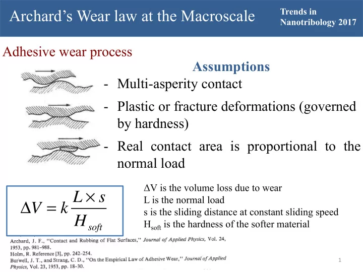
Trends in Archard’s Wear law at the Macroscale Nanotribology 2017 ¡ Adhesive wear process Assumptions - Multi-asperity contact - Plastic or fracture deformations (governed by hardness) - Real contact area is proportional to the normal load Δ V is the volume loss due to wear Δ V = k L × s L is the normal load s is the sliding distance at constant sliding speed H soft H soft is the hardness of the softer material 1 ¡

Trends in Archard’s Wear law at the Macroscale Nanotribology 2017 ¡ Steady-state Running-in Δ V ¡ Δ V is the wear volume ¡ Classical view of s l o p e i s t h e Archard’s law: volumetric wear Barwell’s law: rate Δ V steady − state = k L × t ⎛ ⎞ ⎛ ⎞ Δ V running − in = w 0 τ w 1 − exp − t ⎜ ⎜ ⎟ ⎟ H soft τ w ⎝ ⎠ ⎝ ⎠ F. ¡T. ¡Barwell, ¡Wear ¡1, ¡317 ¡(1958). ¡ t (duration of wear ) Δ V steady − state In the Archard’s law, the wear rate, is s independent of the sliding speed, if the sliding distance, s, is kept constant. 2 ¡

Atomistic wear in a single asperity Trends in Nanotribology 2017 sliding contact ¡ Wear of a Silicon AFM probe on a polymer surface 16 a) c) 14 60 12 pulloff force (nN) tip radius (nm) 10 40 data 8 Archard fit free exponent fit 6 b) 20 4 2 0 0 0 200 400 600 800 sliding distance (m) “Wear occurs through an atom by atom removal process which implies the breaking of individual bonds” 3 ¡ B. ¡Gotsmann ¡and ¡M. ¡A. ¡Lantz, ¡ PRL ¡101, ¡125501 ¡(2008) ¡

Trends in Atomistic Simulation of NanoWear Nanotribology 2017 ¡ D w d � ¼ l � ð s 2 j = G Þ a ? b c Molinari ¡et ¡al. ¡Nature ¡CommunicaLons, ¡11816, ¡(2016) ¡ 4 ¡

Trends in NanoWear Experiments with the AFM Nanotribology 2017 ¡ - Single asperity contact • Main advantage: • Limitations: - N o n c o n s t a n t a n d continuous sliding speed - L o w s l i d i n g s p e e d (typically max.100 µ m/s) - Scan drift leads to non well defined wear track 5 ¡

Trends in Wear Experiments using the CM-AFM Nanotribology 2017 ¡ H.Nasrallah, ¡P-­‑E ¡Mazeran, ¡O.Noel. ¡Rev. ¡Sci. ¡Instrum. ¡ 2011, ¡82, ¡113703. ¡ ¡ Conven&onal)Mode) CM,AFM) Solicita(on*velocity* Low*scanning*or*sliding*velocity** High*sliding*velocity** (typically,*ranging*from*1*µm/s*to*100*µm/s)* (>*6*mm/s)* Advantages*/* High)scanner)dri1;)Low)wear;) Limi(ng*scanner*driC;* Drawbacks) high)shear)force)when)the)scan)changes)its) high*wear*in*a*limi(ng* direc7on) (me;*wellEdefined* wear*track;*isotropic* wear*of*the*probe*if* any;*anisotropic*wear* revealed*if*any;*local* probing*** 6 ¡

Trends in Wear volume computation Nanotribology 2017 ¡ Topography before Topography after Difference wear wear 3 wear image Height (nm) Averaged height of the -2 wear track obtained with a sharp (40 nm of radius) AFM probe -7 1000 1200 1400 1600 1800 Distance from wear track center (nm) 7 ¡

Comparative analysis of Macro and Trends in Nanotribology 2017 Nano wear of copper based composite ¡ Processing Method: Powder Metallurgy SEM and EDX images followed by internal oxidation Designation Average Sample Micro size roughness Hardness particules Rq V 50 Nano- Less than 4.02 nm 224 composite 100 nm AFM image 5 µ m X 5 µ m Amount of nanoparticles FricLon ¡coefficient ¡with ¡steel ¡is ¡0.13 ¡in ¡the ¡steady-­‑state ¡and ¡is ¡ 4.7 wt% and 10% in volume independent ¡of ¡the ¡sliding ¡speed ¡ SEM image of wear track after the ! At the macro-scale, macro tests wear of the nano- (1 N; 8 mm/s) composite follows Mostly adhesive and Archard wear laws light abrasive wear 8 ¡

Trends in Heterogeneity of Nano-wear Nanotribology 2017 ¡ Black&spots& White&spot& 9 ¡

Wear Volume vs. Sliding Distance Trends in Nanotribology 2017 (or wear duration) ¡ Sliding speed of 0.88 mm/s; Normal load = 3 µ N; Diamond Probe t = 2 min. t = 4 min. t = 1 min. t = 8 min. t = 16 min. t = 32 min. 10 ¡

Trends in Wear Volume vs. Sliding Distance Nanotribology 2017 ¡ Si 3 N 4 Probe radius: 100 nm DLC Probe radius: 200 nm like behavior like behavior like behavior like behavior - SEM images do not evidence wear of the probes (counter body). - In both cases, we have an asymptotic steady-state 11 ¡

Trends in Wear volume vs. Normal Load Nanotribology 2017 ¡ 70 nN 100 nN 140 nN 200 nN 12 ¡

Trends in Wear volume vs. Normal Load Nanotribology 2017 ¡ Experiments ¡performed ¡in ¡the ¡running-­‑in-­‑like ¡regime ¡if ¡we ¡refer ¡to ¡a ¡macroscopic ¡view ¡of ¡wear ¡ ¡ DLC probe radius: 200 nm Si 3 N 4 probe radius: 100 nm 7 1.4 Wear,volume,×,10 6 ,,nm 3 Wear*volume*×*10 6 ,*nm 3 Tip:,Si 3 N 4 Tip:*DLC 5.77 6 1.2 1.11 Speed:,0.88,mm/s Speed:*0.88*mm/s Distance:,106,mm Distance:*106*mm 5 1.0 4 0.8 3.00 , 3 0.6 2 0.4 1.42 0.30 slope = 0.04 (10 6 nm 3 .nN) 1 0.2 0.23 slope = 4 (10 6 nm 3 .nN) 0 0.0 0 30 60 90 120 150 180 210 0.0 0.5 1.0 1.5 2.0 2.5 3.0 3.5 ! Normal,load,,nN ! Normal*load,*µN - Archard-like wear law is obtained. - Wear depends on the nature of the counter-body. - For Si 3 N 4 there is a critical threshold load (about 60 nN) from which wear loss is significant. - If we consider a single asperity contact, this latter behavior is governed by the 13 ¡ lateral force which is proportional to the normal load. Eder ¡et ¡al., ¡PRL, ¡115, ¡025502 ¡(2015) ¡

Estimation of the threshold normal Trends in Nanotribology 2017 load ¡ • For a probe radius, R = 100 nm, and a normal load, L = 60 nN (threshold value for SiN probe), the contact radius (Hertz model), a, is: a = 4 nm and the contact pressure is 1.20 GPa < H of sample 2.45 GPa (Hardness of copper oxide is 4-5 GPa). • According to the Hertz theory, the shear stress is maximum at a depth of 0.78 a = 3 nm. This depth corresponds to the thickness of oxide copper growths in ambient conditions. • Therefore, 60 nN corresponds exactly to the normal load that generates a maximum shear stress at a depth of 3 nm. • The threshold value may correspond to the minimum load to apply to shear the interface of the oxide/metal interface. 14 ¡

Trends in Wear Volume vs. sliding speed Nanotribology 2017 ¡ DLC Probe radius: 200 nm Si 3 N 4 Probe radius: 100 nm 40 10 38.21 Wear,rate,×,10 3 ,,nm 3 /mm Wear,rate,×,10 3 ,,nm 3 /mm Tip:,DLC Tip:,Si 3 N 4 9 35 Load:,1,µN Load:,100,nN 8 30 Distance:,317,mm Distance:,106,–,739,mm 7 6.42 5.98 5.96 25 6 Running-in Steady-state 5.84 5.81 20 5 4.72 , 4 15 3.56 3 11.72 9.28 10 2 At the border of the steady-state 3.90 3.64 3.39 3.24 5 1 0 0 0.2 0.4 0.6 0.8 1.0 1.2 1.4 1.6 0.2 0.4 0.6 0.8 1.0 1.2 1.4 1.6 1.8 ! ! Sliding,speed,,mm/s Sliding,speed,,mm/s - Wear rate is independent of the sliding speed (for a given sliding distance et a given normal load) in the steady-state (from the macroscopic view) regime. 15 ¡

Trends in Conclusions and perspectives Nanotribology 2017 ¡ • The methodology based on the CM-AFM gives well-defined wear tracks as the drift of the scanner is limited and the wear loss is significant. • Well defined wear tracks allows measuring quantitative values. • Nano-wear heterogeneity is revealed. Nano-wear of nano-composite, • Archard-like wear laws are revealed at the nanoscale but it does not mean we have the same mechanisms involved as for the macroscale • Wear process may be not governed by the hardness but by the lateral force (or shear stress) and by the physico-chemical interactions in the contact (depending on the nature of the counter-body) • Can we still think in the same way as for the macroscopic view (running-in, steady-state…) ? 16 ¡

Pure copper Wear loss vs. sliding distance Trends in Nanotribology 2017 ¡ 4500 ¡ Wear loss 4000 ¡ 3500 ¡ 3000 ¡ 2500 ¡ 2000 ¡ 1500 ¡ 1000 ¡ 500 ¡ 0 ¡ 0 ¡ 200 ¡ 400 ¡ 600 ¡ 800 ¡ 1000 ¡ 1200 ¡ 1400 ¡ 1600 ¡ Sliding ¡distance, ¡mm ¡ 17 ¡