
SLIDE 1
1.
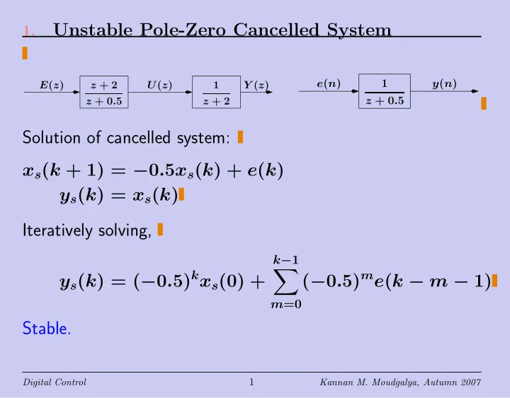
Unstable Pole-Zero Cancelled System
U(z) Y (z) E(z) z + 2 z + 0.5 1 z + 2
y(n) e(n) 1 z + 0.5
Solution of cancelled system: xs(k + 1) = −0.5xs(k) + e(k) ys(k) = xs(k) Iteratively solving, ys(k) = (−0.5)kxs(0) +
k−1
- m=0