Undirected Graphical Models Undirected Graphs Chris Williams, - - PowerPoint PPT Presentation

Undirected Graphical Models

Chris Williams, School of Informatics, University of Edinburgh Overview

• Undirected graphs
• Conditional independence
• Potential functions, energy functions
• Examples: multivariate Gaussian, MRF
• Boltzmann machines, learning rule
• Reading: Jordan section 2.2. [chs 19, 20 for additional reading (not examinable)]

Undirected Graphs

• graph G = (X, E)
• X is a set of nodes, in one-to-
• ne correspondence with a set
• f random variables
• E is a set of undirected edges

between the nodes

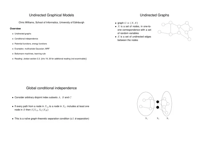
Global conditional independence

• Consider arbitrary disjoint index subsets A, B and C
• If every path from a node in XA to a node in XC includes at least one

node in B then I(XA, XC|XB)

• This is a na¨

ıve graph-theoretic separation condition (c.f. d-separation)

• ✁

X X X

A B C

Graphs and Cliques

• For directed graphs use P(X) =

i P(Xi|Pai), gives notion of locality

• For undirected graphs, locality depends on the notion of cliques
• A clique of a graph is a fully-connected set of nodes
• A maximal clique is a clique which cannot be extended to include

additional nodes without losing the property of being fully connected

Parameterization

• Conditional independence properties of undirected graphs imply a representation of the

joint probability as a product of local functions defined on the maximal cliques of the graph p(x) = 1 Z

• C∈C

ψXC(xc) with Z =

• x
• C∈C

ψXC(xc)

• Each ψXC(xC) is a strictly positive, real-valued function, otherwise arbitrary
• Z is called the partition function
• Equivalence of conditional independence and clique factorization form is the

Hammersley-Clifford theorem ψ (x1,x2) ψ (x1,x3) ψ (x3,x5) ψ (x2,x5,x6) ψ (x2,x4) P(x) = /Z

X X X X X X

1 2 6 3 5 4

• Potential functions are in general neither conditional or marginal

probabilities

• Natural interpretation as agreement, constraint, energy
• Potential function favours certain local configurations by assigning them

larger values

• Global configurations that have high probability are, roughly speaking,

those that satisfy as many of the favoured local configurations as possible

Energy functions

• Enforce positivity by defining

ψXC(xC) = exp{−HXC(xC)}

• Negative sign is conventional (high probability, low energy)

p(x) = 1 Z

• C∈C

ψXC(xc) = 1 Z exp{−

• C∈C

HXC(xC)}

• Energy H(x) =

C∈C HXC(xC)

• Boltzmann distribution

p(x) = 1 Z exp{−H(x)}

Local Markov Property

• Denote all nodes by V
• For a vertex a, let ∂a denote the boundary of a, i.e. the set of vertices in

V \a that are neighbours of a

• Local Markov property: For any vertex a, the conditional distribution of

Xa given XV \a depends only on X∂a

ψ (x1,x2) ψ (x1,x3) ψ (x3,x5) ψ (x2,x5,x6) ψ (x2,x4) P(x) = /Z

X X X X X X

1 2 6 3 5 4

Example I—Multivariate Gaussian

p(x) ∝ exp{−1 2xTΣ−1x}

• It is the zeros in Σ−1 that define the missing edges in the graph and

hence the conditional independence structure

Example II—Markov Random Field

• Discrete random variables
• Ising

model in statistical physics (spins up/down)

• MRF models used in image

analysis, e.g. segmentation of

• regions. Define energies such

that blocks of the same labels are preferred (Geman and Ge- man, 1984)

Boltzmann machines

• Hinton and Sejnowski, 1983
• Binary units ±1

p(x) = 1 Z exp{1 2

• ij

wijxixj}

• wij = wji and wii = 0
• set x0 = 1 (bias unit)
• 1

2

• ij wijxixj =

i<j wijxixj

• Can have hidden units
• Potential function is not arbitrary function of cliques, but only based on

pairwise links (can generalize)

• P(Xi = 1|rest) = σ(2hi) where hi =

j wijxj

hidden units

• utput (visible)

units

Boltzmann machine learning rule

Denote visible units by x, hidden units by y p(x, y) = 1 Z exp{

• k

θkφk(x, y)} This is the general form of a log linear model.

• Features φk(x, y) are the pairwise potentials for a Boltzmann machine
• Parameters θk correspond to weights in the Boltzmann machine

p(x, y) = 1 Z exp{

• k

θkφk(x, y)} p(x) = 1 Z

• y

exp{

• k

θkφk(x, y)} log p(x) = log

• y

exp{

• k

θkφk(x, y)} − log Z ∂log p(x) ∂θl =

• y

φl(x, y)p(y|x) −

• x,y

φl(x, y)p(x, y)

def

= φl(x, y)+ − φl(x, y)−

• + denotes the clamped phase (with x clamped on visible units), −

denotes the free-running phase (all unclamped)

• Learning stops when statistics match in both phases
• Statistics could be computed exactly (using junction tree algorithm) but
• ften this is intractable—

use stochastic sampling

• Boltzmann machine learning rule is gradient based; one can also use

Iterative Scaling algorithms (see Jordan ch 20) to update θk’s

Gibbs sampler

Loop T times for each unit i to be sampled from compute hi and sample P(Xi|rest) end for end loop

• This is a Markov Chain Monte Carlo (MCMC) method. Under general conditions this will

converge to the correct distribution as T → ∞

• Boltzmann machine learning can be slow due to the need to use MCMC techniques.

Gradient is the difference of two noisy estimates

• Hinton (1999, 2000) has introduced the Products of Experts (PoE) architecture, which

may get round some of these difficulties