Two types of GMs Directed edges give causality relationships ( - - PDF document

1

1

School of Computer Science

Undirected Graphical Models

Probabilistic Graphical Models (10 Probabilistic Graphical Models (10-

• 708)

708)

Lecture 2, Sep 17, 2007

Eric Xing Eric Xing

Receptor A Kinase C TF F Gene G Gene H Kinase E Kinase D Receptor B X1 X2 X3 X4 X5 X6 X7 X8 Receptor A Kinase C TF F Gene G Gene H Kinase E Kinase D Receptor B X1 X2 X3 X4 X5 X6 X7 X8 X1 X2 X3 X4 X5 X6 X7 X8

Reading: MJ-Chap. 2,4, and KF-chap5

Eric Xing 2

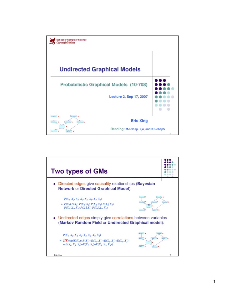
Directed edges give causality relationships (Bayesian

Network or Directed Graphical Model):

Undirected edges simply give correlations between variables

(Markov Random Field or Undirected Graphical model):

Two types of GMs

Receptor A Kinase C TF F Gene G Gene H Kinase E Kinase D Receptor B X1 X2 X3 X4 X5 X6 X7 X8 Receptor A Kinase C TF F Gene G Gene H Kinase E Kinase D Receptor B X1 X2 X3 X4 X5 X6 X7 X8 X1 X2 X3 X4 X5 X6 X7 X8 Receptor A Kinase C TF F Gene G Gene H Kinase E Kinase D Receptor B X1 X2 X3 X4 X5 X6 X7 X8 Receptor A Kinase C TF F Gene G Gene H Kinase E Kinase D Receptor B X1 X2 X3 X4 X5 X6 X7 X8 X1 X2 X3 X4 X5 X6 X7 X8

P(X1, X2, X3, X4, X5, X6, X7, X8) = P(X1) P(X2) P(X3| X1) P(X4| X2) P(X5| X2) P(X6| X3, X4) P(X7| X6) P(X8| X5, X6) P(X1, X2, X3, X4, X5, X6, X7, X8) = 1/Z exp{E(X1)+E(X2)+E(X3, X1)+E(X4, X2)+E(X5, X2) + E(X6, X3, X4)+E(X7, X6)+E(X8, X5, X6)}

2

Eric Xing 3

Review: independence properties

• f DAGs

Defn: let Il(G) be the set of local independence properties

encoded by DAG G, namely:

{ Xi ⊥ NonDescendants(Xi) | Parents(Xi) }

Defn: A DAG G is an I-map (independence-map) of P

if Il(G)⊆ I(P)

A fully connected DAG G is an I-map for any distribution,

since Il(G)=∅⊆ I(P) for any P.

Defn: A DAG G is a minimal I-map for P if it is an I-map for P,

and if the removal of even a single edge from G renders it not an I-map.

A distribution may have several minimal I-maps

• Each corresponding to a specific node-ordering

Eric Xing 4

P-maps

Defn: A DAG G is a perfect map (P-map) for a distribution P if

I(P)=I(G).

Thm: not every distribution has a perfect map as DAG.

• Pf by counterexample. Suppose we have a model where

A ⊥C | {B,D}, and B ⊥D | {A,C}. This cannot be represented by any Bayes net.

• e.g., BN1 wrongly says B ⊥D | A, BN2 wrongly says B ⊥D.

A C C D D B B C A A D D B B BN1 BN1 BN2 BN2 A C C D D B B MRF MRF

3

Eric Xing 5

Undirected graphical models

Pairwise (non-causal) relationships Can write down model, and score specific configurations of

the graph, but no explicit way to generate samples

Contingency constrains on node configurations

X1 X4 X2 X3 X5

Eric Xing 6

Canonical examples

The grid model Naturally arises in image processing, lattice physics, etc. Each node may represent a single "pixel", or an atom

• The states of adjacent or nearby nodes are "coupled" due to pattern continuity or

electro-magnetic force, etc.

• Most likely joint-configurations usually correspond to a "low-energy" state

4

Eric Xing 7

Social networks

The New Testament Social Networks

Eric Xing 8

Protein interaction networks

5

Eric Xing 9

Modeling Go

Eric Xing 10

Information retrieval

topic topic text text image image

6

Eric Xing 11

First hw out today! Start now! Auditing students: please fill out forms Recitation: questions:

Eric Xing 12

Distributional equivalence and I- equivalence

• All independence in Id(G) will be captured in If(G), is the reverse

true?

• Are "not-independence" from G all honored in Pf ?

7

Eric Xing 13

Global Markov Independencies

Let H be an undirected graph: B separates A and C if every path from a node in A to a node

in C passes through a node in B:

A probability distribution satisfies the global Markov property

if for any disjoint A, B, C, such that B separates A and C, A is independent of C given B:

) ; ( sep B C A

H

{ }

) ; ( sep : ) ( I B C A B C A H

H

⊥ =

Eric Xing 14

Soundness of separation criterion

The independencies in I(H) are precisely those that are

guaranteed to hold for every MRF distribution P over H.

In other words, the separation criterion is sound for detecting

independence properties in MRF distributions over H.

8

Eric Xing 15

Local Markov independencies

For each node Xi ∈ V, there is unique Markov blanket of Xi,

denoted MBXi, which is the set of neighbors of Xi in the graph (those that share an edge with Xi)

Defn (5.5.4):

The local Markov independencies associated with H is: Iℓ(H): {Xi ⊥ V – {Xi } – MBXi | MBXi : ∀ i), In other words, Xi is independent of the rest of the nodes in the graph given its immediate neighbors

Eric Xing 16

Structure: an undirected graph

• Meaning: a node is

conditionally independent of every other node in the network given its Directed neighbors

• Local contingency functions

(potentials) and the cliques in the graph completely determine the joint dist.

• Give correlations between

variables, but no explicit way to generate samples

X Y1 Y2

Summary: Conditional Independence Semantics in an MRF

9

Eric Xing 17

Cliques

For G={V,E}, a complete subgraph (clique) is a subgraph

G'={V'⊆V,E'⊆E} such that nodes in V' are fully interconnected

• A (maximal) clique is a complete subgraph s.t. any superset

V"⊃V' is not complete.

• A sub-clique is a not-necessarily-maximal clique.

Example:

• max-cliques = {A,B,D}, {B,C,D},
• sub-cliques = {A,B}, {C,D}, … all edges and singletons

A C C D D B B

Eric Xing 18

Quantitative Specification

Defn: an undirected graphical model represents a distribution

P(X1 ,…,Xn) defined by an undirected graph H, and a set of positive potential functions ψc associated with cliques of H, s.t.

where Z is known as the partition function:

Also known as Markov Random Fields, Markov networks … The potential function can be understood as an contingency

function of its arguments assigning "pre-probabilistic" score of their joint configuration.

∏

∈

=

C c c c n

Z x x P ) ( ) , , ( x ψ 1

1 K

∑ ∏

∈

=

n

x x C c c c

Z

, ,

) (

K

1

x ψ

(A Gibbs distribution)

10

Eric Xing 19

Interpretation of Clique Potentials

The model implies X⊥Z|Y. This independence statement

implies (by definition) that the joint must factorize as:

We can write this as: , but

• cannot have all potentials be marginals
• cannot have all potentials be conditionals

The positive clique potentials can only be thought of as

general "compatibility", "goodness" or "happiness" functions

• ver their variables, but not as probability distributions.

) | ( ) | ( ) ( ) , , ( y z p y x p y p z y x p =

Y X X Z Z ) , ( ) | ( ) , , ( ) | ( ) , ( ) , , ( y z p y x p z y x p y z p y x p z y x p = =

Eric Xing 20

For discrete nodes, we can represent P(X1:4) as two 3D tables

instead of one 4D table

Example UGM – using max cliques

A C C D D B B

) ( ) ( ) , , , ( '

234 124 4 3 2 1

1 x x

c c

Z x x x x P ψ ψ × =

∑

× =

4 3 2 1

234 124 x x x x c c

Z

, , ,

) ( ) ( x x ψ ψ

A,B,D B,C,D

) (

124

x

c

ψ ) (

234

x

c

ψ

11

Eric Xing 21

• We can represent P(X1:4) as 5 2D tables instead of one 4D table
• Pair MRFs, a popular and simple special case
• I(P') vs. I(P") ?

D(P') vs. D(P")

Example UGM – using subcliques

A C C D D B B ) ( ) ( ) ( ) ( ) ( ) ( ) , , , ( "

34 34 24 24 23 23 14 14 12 12 4 3 2 1

1 1 x x x x x x ψ ψ ψ ψ ψ ψ Z Z x x x x P

ij ij ij

= = ∏

∑ ∏

=

4 3 2 1

x x x x ij ij ij

Z

, , ,

) (x ψ

A,B A,D B,D C,D B,C

Eric Xing 22

Factored graph

A C C D D B B

12

Eric Xing 23

Example UGM – canonical representation

A C C D D B B

) ( ) ( ) ( ) ( ) ( ) ( ) ( ) ( ) ( ) ( ) ( ) , , , (

4 4 3 3 2 2 1 1 34 34 24 24 23 23 14 14 12 12 234 124 4 3 2 1

1 x x x x Z x x x x P

c c

ψ ψ ψ ψ ψ ψ ψ ψ ψ ψ ψ × × × = x x x x x x x

∑

× × × =

4 3 2 1

4 4 3 3 2 2 1 1 34 34 24 24 23 23 14 14 12 12 234 124 x x x x c c

x x x x Z

, , ,

) ( ) ( ) ( ) ( ) ( ) ( ) ( ) ( ) ( ) ( ) ( ψ ψ ψ ψ ψ ψ ψ ψ ψ ψ ψ x x x x x x x

• Most general, subsume P' and P" as special cases
• I(P) vs. I(P') vs. I(P")

D(P) vs. D(P') vs. D(P")

Eric Xing 24

Hammersley-Clifford Theorem

• If arbitrary potentials are utilized in the following product formula for

probabilities, then the family of probability distributions obtained is exactly that set which respects the qualitative specification (the conditional independence relations) described earlier

• Thm (5.4.2): Let P be a positive distribution over V, and H a Markov

network graph over V. If H is an I-map for P, then P is a Gibbs distribution over H.

∏

∈

=

C c c c n

Z x x P ) ( ) , , ( x ψ 1

1 K

∑ ∏

∈

=

n

x x C c c c

Z

, ,

) (

K

1

x ψ

13

Eric Xing 25

Independence properties of UGM

Let us return to the question of what kinds of distributions can

be represented by undirected graphs (ignoring the details of the particular parameterization).

Defn: the global Markov properties of a UG H are Is this definition sound and complete?

Y Y Z Z X X

{ }

) ; ( sep : ) ) ( I Y Z X Y Z X H

H

⊥ =

Eric Xing 26

Soundness and completeness of global Markov property

Defn: An UG H is an I-map for a distribution P if I(H) ⊆ I(P),

i.e., P entails I(H).

Defn: P is a Gibbs distribution over H if it can be represented

as

Thm 5.4.1 (soundness): If P is a Gibbs distribution over H,

then H is an I-map of P.

Thm 5.4.5 (completeness): If ¬sepH(X; Z |Y), then X ⊥P Z |Y in

some P that factorizes over H.

∏

∈

=

C c c c n

Z x x P ) ( ) , , ( x ψ 1

1 K

14

Eric Xing 27

Local and global Markov properties revisit

For directed graphs, we defined I-maps in terms of local

Markov properties, and derived global independence.

For undirected graphs, we defined I-maps in terms of global

Markov properties, and will now derive local independence.

Defn: The pairwise Markov independencies associated with

UG H = (V;E) are

e.g.,

{ }

E Y X Y X V Y X H

p

∉ ⊥ = } , { : } , { \ ) ( I } , , {

4 3 2 5 1

X X X X X ⊥

1 1 2 2 3 3 4 4 5 5

Eric Xing 28

Local Markov properties

A distribution has the local Markov property w.r.t. a graph

H=(V,E) if the conditional distribution of variable given its neighbors is independent of the remaining nodes

Theorem (Hammersley-Clifford): If the distribution is strictly

positive and satisfies the local Markov property, then it factorizes with respect to the graph.

NH(X) is also called the Markov blanket of X.

( )

{ }

V V ∈ ∪ ⊥ = X X N X N X X H

H H l

: )) ( ) ( \ ) ( I

15

Eric Xing 29

Relationship between local and global Markov properties

• Thm 5.5.5. If P |= Il(H) then P |= Ip(H).
• Thm 5.5.6. If P = I(H) then P |= Il(H).
• Thm 5.5.7. If P > 0 and P |= Ip(H), then P |= I(H).
• Pf sketch: p(a,b|c,d)=p(a|c,d)p(b|c,d), then d separate b from {a,c}

p(a,b|c,d)p(c|d)=p(a|c,d)p(b|c,d)p(c|d)=p(a,c|d)p(b|d)

• Corollary (5.5.8): The following three statements are equivalent for

a positive distribution P:

P |= Il(H) P |= Ip(H) P |= I(H)

• This equivalence relies on the positivity assumption.
• We can design a distribution locally

Eric Xing 30

I-maps for undirected graphs

Defn: A Markov network H is a minimal I-map for P if it is an I-

map, and if the removal of any edge from H renders it not an I-map.

How can we construct a minimal I-map from a positive

distribution P?

• Pairwise method: add edges between all pairs X,Y s.t.
• Local method: add edges between X and all Y ∈MBP(X), where MBP(X)

is the minimal set of nodes U s.t.

• Thm 5.5.11/12: both methods induce the unique minimal I-map.

If ∃x s.t. P(x) = 0, then we can construct an example where

either method fails to induce an I-map.

( )

} , { \ | Y X V Y X P ⊥ ≠

( )

Y U X V X P | \ } { \ ⊥ ≠ | |

16

Eric Xing 31

Perfect maps

Defn: A Markov network H is a perfect map for P if for any X;

Y;Z we have that

Thm: not every distribution has a perfect map as UGM.

• Pf by counterexample. No undirected network can capture all and only

the independencies encoded in a v-structure X Z Y .

( )

Y Z X P Y Z X

H

| ) ; ( sep ⊥ = ⇔

|

Eric Xing 32

Exponential Form

• Constraining clique potentials to be positive could be inconvenient (e.g.,

the interactions between a pair of atoms can be either attractive or repulsive). We represent a clique potential ψc(xc) in an unconstrained form using a real-value "energy" function φc(xc):

For convenience, we will call φc(xc) a potential when no confusion arises from the context.

• This gives the joint a nice additive strcuture

where the sum in the exponent is called the "free energy": In physics, this is called the "Boltzmann distribution". In statistics, this is called a log-linear model.

{ }

) ( exp ) (

c c c c

x x φ ψ − =

{ }

) ( exp ) ( exp ) ( x x x H Z Z p

C c c c

− = ⎭ ⎬ ⎫ ⎩ ⎨ ⎧− =

∑

∈

1 1 φ

∑

∈

=

C c c c

H ) ( ) ( x x φ

17

Eric Xing 33

Example: Boltzmann machines

A fully connected graph with pairwise (edge) potentials on

binary-valued nodes (for ) is called a Boltzmann machine

Hence the overall energy function has the form:

1 3 3 4 4 2 2

{ } { }

1 1 1 ,

• r

, ∈ + − ∈

i i

x x

⎭ ⎬ ⎫ ⎩ ⎨ ⎧ + + = ⎭ ⎬ ⎫ ⎩ ⎨ ⎧ =

∑ ∑ ∑

C x x x Z x x Z x x x x P

i i i ij j i ij ij j i ij

α θ φ exp ) ( exp ) , , , (

,

1 1

4 3 2 1

) ( ) ( ) ( ) ( ) ( µ µ µ µ − Θ − = − Θ − =∑ x x x x x H

T ij j ij i Eric Xing 34

Example: Ising models

Nodes are arranged in a regular topology (often a regular

packing grid) and connected only to their geometric neighbors.

Same as sparse Boltzmann machine, where θij≠0 iff i,j are

neighbors.

• e.g., nodes are pixels, potential function encourages nearby pixels to

have similar intensities.

Potts model: multi-state Ising model.

⎭ ⎬ ⎫ ⎩ ⎨ ⎧ + =

∑ ∑

∈ i i i N j i j i ij

X X X Z X p

i

,

exp 1 ) ( θ θ

18

Eric Xing 35

Application: Modeling Go

Eric Xing 36

Example: multivariate Gaussian Distribution

A Gaussian distribution can be represented by a fully

connected graph with pairwise (edge) potentials over continuous nodes.

The overall energy has the form

where µ is the mean and Θ is the inverse covariance (precision) matrix.

Also known as Gaussian graphical model (GGM), same as

Boltzmann machine except xi ∈R ) ( ) ( ) ( ) ( ) (

1 1

µ µ µ µ − Σ − = − Σ − =

− −

∑

x x x x x H

T ij j ij i

19

Eric Xing 37

Sparse precision vs. sparse covariance in GGM

2 1 1 3 3 5 4 4 ⎟ ⎟ ⎟ ⎟ ⎟ ⎟ ⎠ ⎞ ⎜ ⎜ ⎜ ⎜ ⎜ ⎜ ⎝ ⎛ = Σ− 5 9 9 4 8 8 3 7 7 2 6 6 1

1

⎟ ⎟ ⎟ ⎟ ⎟ ⎟ ⎠ ⎞ ⎜ ⎜ ⎜ ⎜ ⎜ ⎜ ⎝ ⎛ − − − − − − − − − − = Σ 08 07 12 03 15 07 04 07 01 08 12 07 10 02 13 03 01 02 03 15 15 08 13 15 10 . . . . . . . . . . . . . . . . . . . . . . . . .

) 5 (

• r

) 1 ( 5 1 1 15 nbrs nbrs

X X X ⊥ ⇔ = Σ−

15 5 1

= Σ ⇔ ⊥ X X ⇒

Eric Xing 38

Example: Conditional Random Fields

⎭ ⎬ ⎫ ⎩ ⎨ ⎧ =

∑

c c c c

y x f x Z x y p ) , ( exp ) , ( 1 ) | ( θ θ

θ

A A A A

X2 X3 X1 XT Y2 Y3 Y1 YT

... ... A A A A

X2 X3 X1 XT Y2 Y3 Y1 YT

... ...

Y1 Y2 Y5

…

X1 … Xn

• Discriminative
• Doesn’t assume that features

are independent

• When labeling Xi future
• bservations are taken into

account

20

Eric Xing 39

Conditional Models

• Conditional probability P(label sequence y | observation sequence x)

rather than joint probability P(y, x)

• Specify the probability of possible label sequences given an observation

sequence

• Allow arbitrary, non-independent features on the observation

sequence X

• The probability of a transition between labels may depend on past

and future observations

• Relax strong independence assumptions in generative models

Eric Xing 40

Conditional Distribution

• If the graph G = (V, E) of Y is a tree, the conditional distribution over

the label sequence Y = y, given X = x, by the Hammersley Clifford theorem of random fields is:

─

x is a data sequence

─

y is a label sequence

─

v is a vertex from vertex set V = set of label random variables

─

e is an edge from edge set E over V

─

fk and gk are given and fixed. gk is a Boolean vertex feature; fk is a Boolean edge feature

─

k is the number of features

─

are parameters to be estimated

─

y|e is the set of components of y defined by edge e

─

y|v is the set of components of y defined by vertex v

1 2 1 2

( , , , ; , , , ); and

n n k k

θ λ λ λ µ µ µ λ µ = L L

(y | x) exp ( , y | ,x) ( , y | ,x)

θ

λ µ

∈ ∈

⎛ ⎞ ∝ + ⎜ ⎟ ⎝ ⎠

∑ ∑

k k e k k v e E,k v V ,k

p f e g v

Y1 Y2 Y5

…

X1 … Xn

21

Eric Xing 41

(y| x) exp ( ,y| ,x) ( ,y| 1 (x) ,x)

θ

λ µ

∈ ∈

⎛ ⎞ = + ⎜ ⎟ ⎝ ⎠

∑ ∑

k k e k k v e E,k v V ,k

p f e g v Z

Conditional Distribution (cont’d)

CRFs use the observation-dependent normalization Z(x) for

the conditional distributions:

• Z(x) is a normalization over the data sequence x

Eric Xing 42

Conditional Random Fields

• Allow arbitrary dependencies
• n input
• Clique dependencies on labels
• Use approximate inference for

general graphs

⎭ ⎬ ⎫ ⎩ ⎨ ⎧ =

∑

c c c c

y x f x Z x y p ) , ( exp ) , ( ) | ( θ θ

θ

1