
SLIDE 1
Transition system
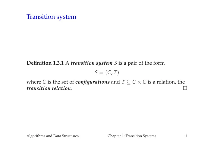
Definition 1.3.1 A transition system S is a pair of the form S
= (C, T )where C is the set of configurations and T
C C is a relation, thetransition relation.
- Algorithms and Data Structures
Chapter 1: Transition Systems 1