Trace Elements in igneous petrology Abundances of trace elements are - - PowerPoint PPT Presentation

Trace Elements in igneous petrology

• Abundances of trace elements are used to test petrogenetic hypotheses
• No universal definition of TE: Concentration usually less than 100 ppm, often < 10 ppm
• Useful trace elements:

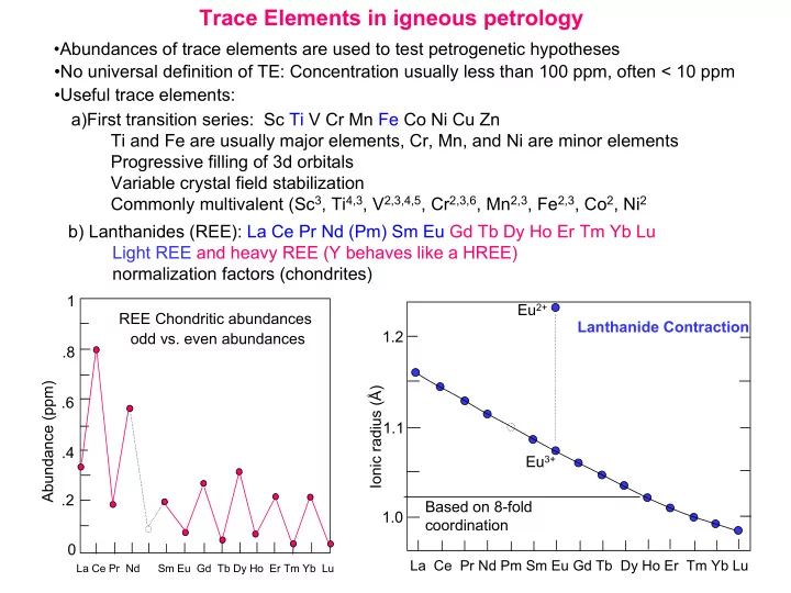
a)First transition series: Sc Ti V Cr Mn Fe Co Ni Cu Zn Ti and Fe are usually major elements, Cr, Mn, and Ni are minor elements Progressive filling of 3d orbitals Variable crystal field stabilization Commonly multivalent (Sc3, Ti4,3, V2,3,4,5, Cr2,3,6, Mn2,3, Fe2,3, Co2, Ni2 b) Lanthanides (REE): La Ce Pr Nd (Pm) Sm Eu Gd Tb Dy Ho Er Tm Yb Lu Light REE and heavy REE (Y behaves like a HREE) normalization factors (chondrites)

Abundance (ppm) 1 .8 .6 .4 .2

La Ce Pr Nd Sm Eu Gd Tb Dy Ho Er Tm Yb Lu

• dd vs. even abundances

REE Chondritic abundances Lanthanide Contraction 1.2 1.1 1.0 Ionic radius (Å) Eu2+ Eu3+ Based on 8-fold coordination

La Ce Pr Nd Pm Sm Eu Gd Tb Dy Ho Er Tm Yb Lu

(c) Large Ion Lithophile Elements (LILE): may also be partitioned into fluid phase Alkalis: K Rb Cs (monovalent) Alkaline earths: Ba Sr (divalent) Actinides: U, Th, Ra, Pa (multiple valency)

• Decoupled from major elements: lack of stoichiometric constraints (not strictly true)
• Generalities: Incompatible elements are elements that tend to be excluded from common

minerals (olivines, pyroxenes, garnets, feldspars, oxides…) in equilibrium with a melt, i.e., they have low D values.

• Numerous exceptions, e.g., Sr, Eu in plag, Cr, Sc in pyroxene, Ni in olivine, HREE in garnet..
• Empirical (not thermodynamic) definition of D (see relevant definitions and equations posted
• n class website)

L i

C

C i

C

L C i

D

/

=

where

L C i

D

/

is the weight distribution coefficient, is concentration (ppm) of trace element i in liquid, and

C i

C

L i

C

is concentration (ppm) of trace element i in the liquid

(d) High field strength elements (HFSE): small, highly-charged ions Zr, Hf (4 valent) Nb, Ta (4 and 5 valent) (e) Chalcophile elements: Cu, Zn, Pb, Ag, Hg, PGE, (Fe, Co, Ni) (f) Siderophile elements: Fe, Ni, Co, Ge, P, Ga, Au (PGE)…

• Goldschmidt’s Rules

L C i

D

/

= Bulk distribution coefficient of i between crystals and liquid = ∑

j j ijW

D

where

j

W

is the weight fraction of mineral j in the solid assemblage

For multiphase crystalline assemblages: Trace elements are used to model processes of melting (equilibrium and fractional) and crystallization (equilibrium and fractional). To model melting processes, two types of melting are considered (1) modal melting where the minerals melt in the same proportions that they are present in the crystal assemblage and (2) non-modal melting in which the minerals melt in proportions controlled by the stoichiometry of the melting reaction, which usually has to be determined experimentally or from a known phase

• diagram. The equations for all types of crystallization and melting are listed on the class

website under: “Trace element definitions and equations”.

L C i

D

/

Distribution coefficients

• Attempts have been made over the past 3 decades to determine the appropriate

values of distribution coefficients to be used in modeling. The earliest attempts simply separated phenocrysts from matrix in volcanic rocks and analyzed each to

• btain an empirical set of D values. Some of these data are still used today.
• More recently experiments have been carried out over a wide range of T, P and X

using a variety of methods. As the techniques of microanalysis of trace element abundances improved (SIMS, LA-ICPMS…), this approach has been popular.

D values are functions of T, P and composition of both crystalline and melt phases so the

problem becomes one of controlling these variables and trying to establish a theoretical basis that would allow one to predict D values based on a limited number of experiments. Only limited success to date so a wide range of D values exist in the literature. Caveat: Be careful about choice of D values used—make sure they are appropriate. This figure on left shows D values for REE that have been used to model processes in mafic magmas. While the D values may vary as functions of T, P, XL and Xxal, the figure clearly show the major differences among common

• minerals. Note the log scale on the Y-axis.

The figure below shows an example of the effect on D values of changing crystal composition

Good source of D values: Table 7.5 in the online book by W. M. White “Geochemistry”

Table 9-1. Partition Coefficients (CS/CL) for Some Commonly Used Trace Elements in Basaltic and Andesitic Rocks Olivine Opx Cpx Garnet Plag Amph Magnetite Rb 0.010 0.022 0.031 0.042 0.071 0.29 Sr 0.014 0.040 0.060 0.012 1.830 0.46 Ba 0.010 0.013 0.026 0.023 0.23 0.42 Ni 14 5 7 0.955 0.01 6.8 29 Cr 0.70 10 34 1.345 0.01 2.00 7.4 La 0.007 0.03 0.056 0.001 0.148 0.544 2 Ce 0.006 0.02 0.092 0.007 0.082 0.843 2 Nd 0.006 0.03 0.230 0.026 0.055 1.340 2 Sm 0.007 0.05 0.445 0.102 0.039 1.804 1 Eu 0.007 0.05 0.474 0.243 0.1/1.5* 1.557 1 Dy 0.013 0.15 0.582 1.940 0.023 2.024 1 Er 0.026 0.23 0.583 4.700 0.020 1.740 1.5 Yb 0.049 0.34 0.542 6.167 0.023 1.642 1.4 Lu 0.045 0.42 0.506 6.950 0.019 1.563

Data from Rollinson (1993). * Eu3+/Eu2+ Italics are estimated

Rare Earth Elements

Table 9-1: from Winter (2001) An introduction to Igneous and metamorphic petrology. Prentice Hall Tables such as this one are useful but they can also be misleading in that they imply that D values are constant for a given element in a given mineral This figure shows the range of values measured experimentally for the distribution coefficient of Ni in

• livine showing the effect on D value of variable

MgO content of the melt. There is also a temperature dependence which is “hidden” in these

• data. The experiments (>10 sets) were carried out

at T ranging from 1600ºC to 1100ºC. Liquid compositions ranged from ultramafic (komatiites) to mafic (basalts). 30 30 10 20 20 10 DNI

• Wt. % MgO in liquid

Olivine/melt D values D values > 1 compatible element D values < 1 incompatible element

In Onuma diagrams, partition coefficients plotted against ionic radius define smooth convex- upward curves with a different curve for each valence. The maximum in the curves predicts the best fit ionic radius. 0.01 1 10 0.1 0.8 1.2 1.4 1.6 1.0

Ionic radius (Å) D

“Onuma” diagram for plagioclase

Mg2+ Ca2+ Sr2+ Ba2+ Lu Yb Sm Ce 3+ Dy

Normalization factors, spider diagrams, etc.

• 1. REE: REE abundances in minerals and rocks are normalized by dividing the

abundances by abundances in C1 chondrites (see table below for typical values)

Ch (ppm) La 0.325 Ce 0.798 Nd 0.567 Sm 0.186 Eu 0.0692 Gd 0.255 Tb 0.047 Dy 0.305 Er 0.209 Yb 0.209 Lu 0.0349

• 2. Spidergrams: abundances of trace elements in minerals and rocks are normalized by dividing

by abundances in the mantle (or MORB or…). Plotted in order of decreasing incompatibility

This figure shows a typical REE normalized plot for basalts. In this example, basalts from the CRB flood basalt province. A pattern like this is said to show a moderate degree of LREE enrichment (La/Yb)N > 1

Data from Hooper and Hawkesworth (1993)

• J. Petrol., 34, 1203-1246. Reproduced in

Winter (2001) An introduction to Igneous and metamorphic petrology. Prentice Hall

MORB-normalized spider diagram for some representative analyses from the CRB flood basalts

Data from Hooper and Hawkesworth (1993)

• J. Petrol., 34, 1203-1246. Reproduced in

Winter (2001). An Introduction to Igneous and Metamorphic Petrology. Prentice Hall

Commonly used normalization factors for spider diagrams are provided by Sun and McDonough (1989)

Example of an equilibrium partial modal melting calculation involving Rb and Sr

Suppose we are melting a lower crustal granulite containing 50% plagioclase + 25% cpx + 20% opx + 5% garnet and we want to track how the Rb, Sr and Rb/Sr concentrations in the melt vary as the melting progresses. Assuming modal batch melting, equation to use is: ) ) 1 ( ( 1

i i L O i L i

D D F C C + − = First, we need to calculate for the crystalline assemblage using White’s D values DSr = (0.5x2.7) + (0.25x0.157) + (0.2x0.0068) + (0.05x.0099) = 1.39 DRb = (0.5x0.025) + (0.25x0.033) + (0.2x0.022) + (0.05x0.007) = 0.025

L C i

D

/

Note: (1) dramatic decrease in Rb and Rb/Sr as melting progresses. (2) Essentially constant Sr during progressive melting. (3) Is it justified to assume constant D values and modal melting?

60 0.4 50 40 30 20 10 0.2 0.3 0.1

• Sr

L Sr

C C

• Rb

L Rb

C C

• Sr
• Rb

L Sr L Rb

C C C C /

FL

0 .72 40.0 55.6 0.02 .723 22.5 31.1 0.05 .73 13.6 18.6 0.1 .74 8.2 11.0 0.2 .76 4.6 6.0 0.3 .79 3.1 4.0 0.4 .81 2.4 3.0

• Sr

L Sr

C C

• Rb

L Rb

C C

FL

• Sr
• Rb

L Sr L Rb

C C C C /

This calculation assumes constant D values