Today CS 188: Artificial Intelligence Neural Nets (wrap-up) and - PowerPoint PPT Presentation

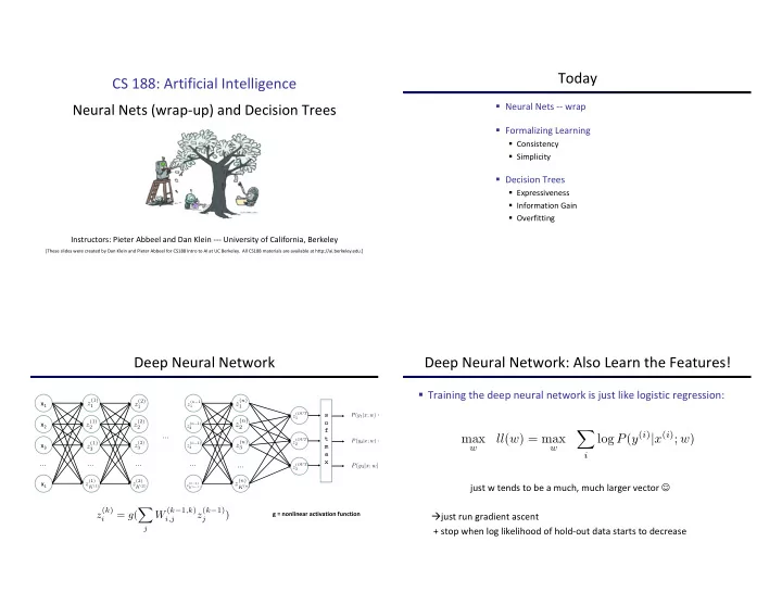
Today CS 188: Artificial Intelligence Neural Nets (wrap-up) and Decision Trees § Neural Nets -- wrap § Formalizing Learning § Consistency § Simplicity § Decision Trees § Expressiveness § Information Gain § Overfitting Instructors: Pieter Abbeel and Dan Klein --- University of California, Berkeley [These slides were created by Dan Klein and Pieter Abbeel for CS188 Intro to AI at UC Berkeley. All CS188 materials are available at http://ai.berkeley.edu.] Deep Neural Network Deep Neural Network: Also Learn the Features! § Training the deep neural network is just like logistic regression: z (1) x 1 z (2) z ( n ) z ( n − 1) 1 1 1 1 z ( OUT ) s P ( y 1 | x ; w ) = 1 z ( n ) z (1) z (2) x 2 o z ( n − 1) 2 2 2 2 f X log P ( y ( i ) | x ( i ) ; w ) … max ll ( w ) = max t z ( OUT ) P ( y 2 | x ; w ) = z ( n ) x 3 z (1) z (2) z ( n − 1) 2 m w w 3 3 3 3 a i x … … … … … z ( OUT ) P ( y 3 | x ; w ) = 3 z (1) z (2) z ( n ) x L z ( n − 1) just w tends to be a much, much larger vector J K (1) K (2) K ( n ) K ( n − 1) z ( k ) W ( k − 1 ,k ) z ( k − 1) X = g ( ) g = nonlinear activation function à just run gradient ascent i i,j j + stop when log likelihood of hold-out data starts to decrease j

Neural Networks Properties How well does it work? § Theorem (Universal Function Approximators). A two-layer neural network with a sufficient number of neurons can approximate any continuous function to any desired accuracy. § Practical considerations § Can be seen as learning the features § Large number of neurons § Danger for overfitting § (hence early stopping!) Computer Vision Object Detection

Manual Feature Design Features and Generalization [HoG: Dalal and Triggs, 2005] Performance Features and Generalization Image HoG graph credit Matt Zeiler, Clarifai

Performance Performance AlexNet graph credit Matt graph credit Matt Zeiler, Clarifai Zeiler, Clarifai Performance Performance AlexNet AlexNet graph credit Matt graph credit Matt Zeiler, Clarifai Zeiler, Clarifai

Visual QA Challenge MS COCO Image Captioning Challenge Stanislaw Antol, Aishwarya Agrawal, Jiasen Lu, Margaret Mitchell, Dhruv Batra, C. Lawrence Zitnick, Devi Parikh Karpathy & Fei-Fei, 2015; Donahue et al., 2015; Xu et al, 2015; many more Speech Recognition Machine Translation Google Neural Machine Translation (in production) graph credit Matt Zeiler, Clarifai

Today Inductive Learning § Neural Nets -- wrap § Formalizing Learning § Consistency § Simplicity § Decision Trees § Expressiveness § Information Gain § Overfitting § Clustering Inductive Learning (Science) Inductive Learning § Curve fitting (regression, function approximation): § Simplest form: learn a function from examples § A target function: g § Examples: input-output pairs ( x , g ( x )) § E.g. x is an email and g ( x ) is spam / ham § E.g. x is a house and g ( x ) is its selling price § Problem: § Given a hypothesis space H § Given a training set of examples x i § Find a hypothesis h ( x ) such that h ~ g § Includes: § Classification (outputs = class labels) § Regression (outputs = real numbers) § Consistency vs. simplicity § How do perceptron and naïve Bayes fit in? ( H , h, g , etc.) § Ockham’s razor

Consistency vs. Simplicity Decision Trees § Fundamental tradeoff: bias vs. variance § Usually algorithms prefer consistency by default (why?) § Several ways to operationalize “simplicity” § Reduce the hypothesis space § Assume more: e.g. independence assumptions, as in naïve Bayes § Have fewer, better features / attributes: feature selection § Other structural limitations (decision lists vs trees) § Regularization § Smoothing: cautious use of small counts § Many other generalization parameters (pruning cutoffs today) § Hypothesis space stays big, but harder to get to the outskirts Reminder: Features Decision Trees § Features, aka attributes § Compact representation of a function: § Sometimes: TYPE=French § Truth table § Sometimes: f TYPE=French ( x ) = 1 § Conditional probability table § Regression values § True function § Realizable: in H

Expressiveness of DTs Comparison: Perceptrons What is the expressiveness of a perceptron over these features? § § Can express any function of the features For a perceptron, a feature’s contribution is either positive or negative § § If you want one feature’s effect to depend on another, you have to add a new conjunction feature § E.g. adding “PATRONS=full Ù WAIT = 60” allows a perceptron to model the interaction between the two atomic features DTs automatically conjoin features / attributes § § Features can have different effects in different branches of the tree! Difference between modeling relative evidence weighting (NB) and complex evidence interaction (DTs) § § Though if the interactions are too complex, may not find the DT greedily § However, we hope for compact trees Hypothesis Spaces Decision Tree Learning § Aim: find a small tree consistent with the training examples How many distinct decision trees with n Boolean attributes? § § Idea: (recursively) choose “most significant” attribute as root of (sub)tree = number of Boolean functions over n attributes = number of distinct truth tables with 2 n rows = 2^(2 n ) E.g., with 6 Boolean attributes, there are § 18,446,744,073,709,551,616 trees How many trees of depth 1 (decision stumps)? § = number of Boolean functions over 1 attribute = number of truth tables with 2 rows, times n = 4n E.g. with 6 Boolean attributes, there are 24 decision stumps § More expressive hypothesis space: § § Increases chance that target function can be expressed (good) Increases number of hypotheses consistent with training set § (bad, why?) Means we can get better predictions (lower bias) § But we may get worse predictions (higher variance) §

Choosing an Attribute Entropy and Information § Idea: a good attribute splits the examples into subsets that are (ideally) “all positive” or § Information answers questions “all negative” § The more uncertain about the answer initially, the more information in the answer § Scale: bits § Answer to Boolean question with prior <1/2, 1/2>? § Answer to 4-way question with prior <1/4, 1/4, 1/4, 1/4>? § Answer to 4-way question with prior <0, 0, 0, 1>? § Answer to 3-way question with prior <1/2, 1/4, 1/4>? § A probability p is typical of: § So: we need a measure of how “good” a split is, even if the results aren’t perfectly § A uniform distribution of size 1/p separated out § A code of length log 1/p Entropy Information Gain § General answer: if prior is < p 1 ,…,p n >: § Back to decision trees! For each split, compare entropy before and after § § Information is the expected code length § Difference is the information gain § Problem: there’s more than one distribution after split! 1 bit § Also called the entropy of the distribution 0 bits § More uniform = higher entropy § More values = higher entropy § Solution: use expected entropy, weighted by the number of § More peaked = lower entropy examples § Rare values almost “don’t count” 0.5 bit

Next Step: Recurse Example: Learned Tree § Now we need to keep growing the tree! § Decision tree learned from these 12 examples: § Two branches are done (why?) § What to do under “full”? § See what examples are there… § Substantially simpler than “true” tree § A more complex hypothesis isn't justified by data § Also: it’s reasonable, but wrong Example: Miles Per Gallon Find the First Split mpg cylinders displacement horsepower weight acceleration modelyear maker § Look at information gain for good 4 low low low high 75to78 asia each attribute bad 6 medium medium medium medium 70to74 america bad 4 medium medium medium low 75to78 europe bad 8 high high high low 70to74 america bad 6 medium medium medium medium 70to74 america 40 Examples bad 4 low medium low medium 70to74 asia bad 4 low medium low low 70to74 asia § Note that each attribute is bad 8 high high high low 75to78 america : : : : : : : : correlated with the target! : : : : : : : : : : : : : : : : bad 8 high high high low 70to74 america good 8 high medium high high 79to83 america bad 8 high high high low 75to78 america § What do we split on? good 4 low low low low 79to83 america bad 6 medium medium medium high 75to78 america good 4 medium low low low 79to83 america good 4 low low medium high 79to83 america bad 8 high high high low 70to74 america good 4 low medium low medium 75to78 europe bad 5 medium medium medium medium 75to78 europe

Result: Decision Stump Second Level Reminder: Overfitting Final Tree § Overfitting: § When you stop modeling the patterns in the training data (which generalize) § And start modeling the noise (which doesn’t) § We had this before: § Naïve Bayes: needed to smooth § Perceptron: early stopping