Time Series Time Series Time Series Prof. Paolo Ciaccia Prof. - PDF document

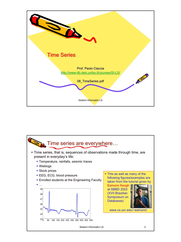
Time Series Time Series Time Series Prof. Paolo Ciaccia Prof. Paolo Ciaccia http://www- http://www -db. db.deis deis. .unibo unibo. .it it/ /courses courses/SI /SI- -LS/ LS/ 08_TimeSeries.pdf 08_TimeSeries. pdf Sistemi Informativi LS Time series are everywhere… � Time series, that is, sequences of observations made through time, are present in everyday’s life: � Temperature, rainfalls, seismic traces � Weblogs � Stock prices � This as well as many of the � EEG, ECG, blood pressure following figures/examples are � Enrolled students at the Engineering Faculty taken from the tutorial given by � … Eamonn Keogh at SBBD 2002 29 (XVII Brazilian 28 Symposium on 27 Databases) 26 25 www.cs.ucr.edu/~eamonn/ 24 23 0 50 100 150 200 250 300 350 400 450 500 Sistemi Informativi LS 2

Why is similarity search in t.s.’s important? � Consider a large time series DB: � 1 hour of ECG data: 1 GByte � Typical Weblog: 5 GBytes per week � Space Shuttle DB: 158 GBytes � MACHO Astronomical DB: 2 TBytes, updated with 3 GBytes a day (20 million stars recorded nightly for 4 years) http://wwwmacho.anu.edu.au/ � Similarity search can help you in: � Looking for the occurrence of known patterns � Discovering unknown patterns � Putting “things together” (clustering) � Classifiying new data � Predicting/extrapolating future behaviors � … Sistemi Informativi LS 3 How to measure similarity � Given two time series of equal length D, the commonest way to measure their (dis-)similarity is based on Euclidean distance � However, with Euclidean distance we have to face two basic problems 1. High-dimensionality: (very) large D values 2. Sensitivity to “alignment of values” s q � For problem 1. we need to define effective lower-bounding techniques that work in a (much) lower dimensional space � For problem 2. we will introduce ( ) D - 1 ( ) = − 2 L s, q ∑ s q a new similarity criterion 2 t t t = 0 Sistemi Informativi LS 4

Dimensionality reduction: DFT (1) � The first approach to reducing the dimensionality of time series, proposed in [AFS93], was based on Discrete Fourier Transform (DFT) � Remind: given a time series s, the Fourier coefficients are complex numbers (amplitude,phase), defined as: 1 D − 1 ( ) ∑ = − = − S s exp j 2 π f t/D f 0,..., D 1 f t D = t 0 � From Parseval theorem we know that DFT preserves the energy of the signal: D − 1 D − 1 ( ) ∑ ( ) ∑ 2 = = = E s s 2 E S S t f = = t 0 f 0 � Since DFT is a linear transformation we have: − − D 1 D 1 ∑ ( ) ( ) ( ) ∑ 2 2 2 = − = − = − = − = 2 L (s, q) s q E s q E S Q S Q L (S, Q) 2 t t f f 2 t = 0 f = 0 thus, DFT preserves the Euclidean distance � And? What can we gain from such transformation?? Sistemi Informativi LS 5 Dimensionality reduction: DFT (2) � The key observation is that, by keeping only a small set of Fourier coefficients, we can obtain a good approximation of the original signal � Why: because most of the energy of many real-world signals concentrates in the low frequencies ([AFS+93]): � More precisely, the energy spectrum (|S f | 2 vs. f) behaves as O(f -b ), b > 0: � b = 2 (random walk or brown noise): used to model the behavior of stock movements and currency exchange rates � b > 2 (black noise): suitable to model slowly varying natural phenomena (e.g., water levels of rivers) � b = 1 (pink noise): according to Birkhoff’s theory, musical scores follow this energy pattern � Thus, if we only keep the first few coefficients (D’ << D) we can achieve an effective dimensionality reduction � Note: this is the basic idea used by well-known compression standards, such as JPEG (which is based on Discrete Cosine Transform) � For what we have seen, this “projection” technique satisfies the L-B lemma Sistemi Informativi LS 6

An example: EEG data � Sampling rate: 128 Hz Energy spectrum Time series (4 secs, 512 points) Sistemi Informativi LS 7 Another example First 4 Fourier Fourier data values coefficients coefficients � 128 points 0.4995 1.5698 1.5698 0.5264 1.0485 1.0485 0.5523 0.7160 0.7160 0.5761 0.8406 0.8406 s 0.5973 0.3709 0.3709 0.6153 0.4670 0.4670 s’ 0.6301 0.2667 0.2667 0.6420 0.1928 0.1928 0.6515 0.1635 0.6596 0.1602 0 20 40 60 80 100 120 140 0.6672 0.0992 0.6751 0.1282 0.6843 0.1438 0.6954 0.1416 0.7086 0.1400 0.7240 0.1412 0.7412 0.1530 0.7595 0.0795 0.7780 0.1013 0.7956 0.1150 0.8115 0.1801 0.8247 0.1082 s’ = approximation of s with 0.8345 0.0812 4 Fourier coefficients 0.8407 0.0347 0.8431 0.0052 0.8423 0.0017 0.8387 0.0002 … ... Sistemi Informativi LS 8

Comments on DFT ☺ Can be computed in O(DlogD) time using FFT (provided D is a power of 2) � Difficult to use if one wants to deal with sequences of different length � Not really amenable to deal with “signals with spots” (time-varying energy) � An alternative to DFT is to use wavelets , which takes a different perspective: � A signal can be represented as a sum of contributions, each at a different resolution level � Discrete Wavelet Transform (DWT) can be computed in O(D) time � Experimental results however show that the superiority of DWT w.r.t. DFT is dependent on the specific dataset Good for Good for wavelets Fourier bad for bad for Fourier wavelets 0 200 400 Sistemi Informativi LS 600 0 200 400 9 600 Dimensionality reduction: PAA � PAA (Piecewise Aggregate Approximation) [KCP+00,YF00] is a very simple, intuitive and fast (O(D)) method to approximate time series � Its performance is comparable to that of DFT and DWT � We take a window of size W and segment our time series into D’ = D/W “pieces” (sub-sequences), each of size W × − i W 1 ∑ s � For each piece, we compute the average of values, i.e. t ( ) = t = i − 1 × W ' � Our approximation is therefore s’ = (s’ 1 ,…,s’ D’ ) s i W � We have √ W × L 2 (s’,q’) ≤ L 2 (s,q) (arguments generalize those used for the “global average” example) � The same can be generalized to work with arbitrary Lp-norms [YF00] s W s' 0 20 40 60 80 100 120 140 Sistemi Informativi LS 10

The “alignment” problem � Euclidean distance, as well as other Lp-norms, are not robust w.r.t., even small, contractions/expansions of the signal along the time axis � E.g., speech signals � Intuitively, we would need a distance measure that is able to “match” a point of time series s even with “surrounding” points of time series q � Alternatively, we may view the time axis as a “stretchable” one � A distance like this exists, and is called “Dynamic Time Warping” (DTW)! Fixed Time Axis “Warped” Time Axis Sequences are aligned “one to one” Non-linear alignments are possible Sistemi Informativi LS 11 How to compute the DTW (1) � Assume that the two time series s and q have the same length D � Note that with DTW this is not necessary anymore! � Construct a D × D matrix d, whose element d i,j is the distance between s i and q j � We take d i,j = (s i - q j ) 2 , but other possibilities exist (e.g., |s i – q j |) D=6 0 1 2 3 4 5 7 25 16 25 36 16 9 s 1 2 5 4 3 7 3 1 0 1 4 0 1 q 2 3 2 1 3 4 4 4 1 4 9 1 0 s L 2 (s,q) = √ 29 5 9 4 9 16 4 1 � The “rules of the game”: 2 0 1 0 1 1 4 � Start from (0,0) and end in (D-1,D-1) 1 1 4 1 0 4 9 � Take one step at a time d 2 3 2 1 3 4 � At each step, move only by increasing i, j, or both q � I.e., never go back! � “Jumps” are not allowed! � Sum all distances you have found in the “warping path” Sistemi Informativi LS 12

How to compute the DTW (2) � The figure shows a possible warping path w, whose “cost” is 21 � The “Euclidean path” moves only along the main diagonal, and costs 29 7 25 16 25 36 16 9 3 1 0 1 4 0 1 4 4 1 4 9 1 0 s 5 9 4 9 16 4 1 2 0 1 0 1 1 4 1 1 4 1 0 4 9 2 3 2 1 3 4 warping path w q The DTW is the minimum cost among all the warping paths � But the number of path is exponential in D � � Ok, but we can use dynamic programming, with complexity O(D 2 ) ☺ Sistemi Informativi LS 13 How to compute the DTW (3) � From the d matrix, incrementally build a new matrix WP, whose elements wp i,j are recursively defined as: = + wp d min{wp , wp , wp } i, j i, j i - 1, j i, j- 1 i - 1, j- 1 7 25 16 25 36 16 9 7 40 22 31 43 24 15 3 1 0 1 4 0 1 3 15 6 7 11 8 6 4 4 1 4 9 1 0 4 14 6 9 18 8 5 s s 5 9 4 9 16 4 1 5 10 5 11 18 7 5 2 0 1 0 1 1 4 2 1 2 2 3 4 8 1 1 4 1 0 4 9 1 1 5 6 6 10 19 d 2 3 2 1 3 4 WP 2 3 2 1 3 4 q q � Then set d DTW (s,q) = √ wp D-1,D-1 Sistemi Informativi LS 14

A real-world graphical example Monday was a holiday Power-Demand time teries Each sequence corresponds to a week’s demand for power Wednesday was a holiday in a Dutch research facility in 1997 Sistemi Informativi LS 15 Fast searching with DTW � We have now 2 problems to face, if we want to use DTW for searching: 1. Computing the DTW is very time-consuming 2. How to index it? � Both problems can be solved: 1. Use a lower-resolution approximation of the time series � However the method can introduce false dismissals 22.7 sec 1.3 sec Sistemi Informativi LS 16