Outline Time series and forecasting Time series objects 1 in R - PDF document

Time series and forecasting in R 1 Time series and forecasting in R 2 Outline Time series and forecasting Time series objects 1 in R Basic time series functionality 2 The forecast package 3 Rob J Hyndman Exponential smoothing 4 ARIMA modelling 5 29 June 2008 More from the forecast package 6 Time series packages on CRAN 7 Time series and forecasting in R Time series objects 4 Time series and forecasting in R Time series objects 5 Australian GDP 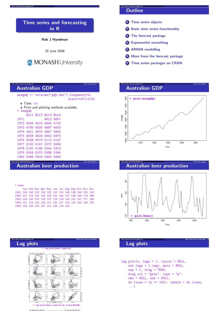Australian GDP ausgdp <- ts(scan("gdp.dat"),frequency=4, 7500 start=1971+2/4) > plot(ausgdp) Class: ts 7000 Print and plotting methods available. > ausgdp 6500 Qtr1 Qtr2 Qtr3 Qtr4 ausgdp 6000 1971 4612 4651 1972 4645 4615 4645 4722 5500 1973 4780 4830 4887 4933 1974 4921 4875 4867 4905 5000 1975 4938 4934 4942 4979 4500 1976 5028 5079 5112 5127 1975 1980 1985 1990 1995 1977 5130 5101 5072 5069 Time 1978 5100 5166 5244 5312 1979 5349 5370 5388 5396 1980 5388 5403 5442 5482 Time series and forecasting in R Time series objects 6 Time series and forecasting in R Time series objects 7 Australian beer production Australian beer production 180 > beer Jan Feb Mar Apr May Jun Jul Aug Sep Oct Nov Dec 1991 164 148 152 144 155 125 153 146 138 190 192 192 160 beer 1992 147 133 163 150 129 131 145 137 138 168 176 188 1993 139 143 150 154 137 129 128 140 143 151 177 184 1994 151 134 164 126 131 125 127 143 143 160 190 182 140 1995 138 136 152 127 151 130 119 153 120 > plot(beer) 1991 1992 1993 1994 1995 Time Time series and forecasting in R Basic time series functionality 9 Time series and forecasting in R Basic time series functionality 10 Lag plots Lag plots > lag.plot(beer,lags=12) 100 120 140 160 180 200 100 120 140 160 180 200 12 11 12 11 11 12 47 10 47 10 47 10 24 24 24 180 36 36 36 48 48 48 35 23 23 35 35 23 22 22 22 160 39 1 15 15 39 1 39 15 1 beer 46 beer 46 beer 46 5 28 28 5 28 5 51 53 37 7 3 34 53 7 51 3 37 34 3 37 51 34 53 7 16 27 16 27 27 16 lag.plot(x, lags = 1, layout = NULL, 13 8 2 2 13 8 13 2 8 140 19 44 26 33 4 45 4 19 26 44 33 45 26 4 19 32 33 45 44 32 32 49 25 21 9 25 49 21 9 49 25 21 9 29 20 50 29 50 20 29 50 20 14 38 38 14 14 38 54 41 30 17 18 41 18 30 17 54 17 18 41 30 31 43 52 52 43 31 52 31 43 120 42 40 6 40 42 6 40 6 42 55 set.lags = 1:lags, main = NULL, lag 1 lag 2 lag 3 12 11 12 11 11 12 10 47 24 47 24 10 24 10 47 36 36 36 180 48 48 48 asp = 1, diag = TRUE, 35 35 35 23 23 23 22 22 22 39 15 1 1 15 39 15 39 1 160 beer beer beer 46 46 46 5 5 5 51 28 3 7 28 3 51 7 3 7 28 27 37 34 16 37 16 27 34 37 34 27 16 2 13 13 2 13 2 diag.col = "gray", type = "p", 4 19 8 4 8 19 8 19 4 140 26 45 33 44 26 45 33 44 44 26 45 33 25 32 25 32 25 32 50 21 29 9 49 20 50 49 9 2021 29 49 20 21 50 9 29 38 14 38 14 14 38 41 18 41 18 18 41 17 30 31 17 30 31 31 17 30 40 52 42 43 6 40 43 42 6 43 40 42 6 120 oma = NULL, ask = NULL, lag 4 lag 5 lag 6 11 12 12 11 12 11 10 47 47 10 10 47 24 24 24 180 36 36 36 48 48 do.lines = (n <= 150), labels = do.lines, 35 23 23 35 23 35 22 22 22 160 39 39 39 1 15 1 15 15 1 beer 46 beer 46 beer 46 28 5 5 28 5 28 34 7 37 3 34 37 7 3 34 7 37 3 2 27 16 27 16 2 16 27 2 13 19 8 13 19 8 8 19 13 ...) 140 33 45 26 44 4 3233 44 45 26 4 33 45 4 44 26 32 32 25 2021 9 49 29 9 21 25 29 20 21 9 29 20 25 38 38 38 14 14 14 18 30 41 17 30 41 1718 41 17 18 30 31 43 40 43 31 40 31 43 40 120 42 6 42 6 42 6 lag 7 lag 8 lag 9 10 11 12 10 11 12 10 11 12 24 24 24 36 36 36 180 35 35 35 23 23 23 22 22 22 15 39 1 39 15 1 1 15 39 160 beer 46 beer beer 5 5 5 7 28 3 7 3 28 28 7 3 16 34 27 37 27 34 16 37 37 16 34 27 8 13 2 8 2 13 2 13 8 4 19 19 4 19 4 140 45 33 44 26 44 33 45 26 26 33 44 32 21 9 25 32 9 21 25 9 32 21 25 20 29 20 29 29 20 38 14 38 14 38 14 1718 41 41 18 18 41 3031 43 31 30 43 17 43 30 31 17 42 40 6 6 42 40 40 42 6 120 lag 10 lag 11 lag 12 100 120 140 160 180 200 > lag.plot(beer,lags=12,do.lines=FALSE) 100 120 140 160 180 200 100 120 140 160 180 200

Time series and forecasting in R Basic time series functionality 11 Time series and forecasting in R Basic time series functionality 12 ACF PACF 1.0 0.4 > pacf(beer) > acf(beer) 0.8 0.6 0.2 Partial ACF 0.4 ACF 0.2 0.0 0.0 −0.2 −0.2 −0.4 0.0 0.2 0.4 0.6 0.8 1.0 1.2 1.4 0.2 0.4 0.6 0.8 1.0 1.2 1.4 Lag Lag Time series and forecasting in R Basic time series functionality 13 Time series and forecasting in R Basic time series functionality 14 ACF/PACF Spectrum Raw periodogram 500.0 > spectrum(beer) 100.0 acf(x, lag.max = NULL, type = c("correlation", "covariance", "partial"), plot = TRUE, na.action = na.fail, demean = TRUE, ...) 20.0 spectrum pacf(x, lag.max, plot, na.action, ...) 5.0 ARMAacf(ar = numeric(0), ma = numeric(0), lag.max = r, 2.0 pacf = FALSE) 0.5 0.2 0 1 2 3 4 5 6 frequency Time series and forecasting in R Basic time series functionality 15 Time series and forecasting in R Basic time series functionality 16 Spectrum Spectrum AR(12) spectrum 1000 > spectrum(beer,method="ar") spectrum(x, ..., method = c("pgram", "ar")) 500 spec.pgram(x, spans = NULL, kernel, taper = 0.1, 200 pad = 0, fast = TRUE, demean = FALSE, spectrum 100 detrend = TRUE, plot = TRUE, na.action = na.fail, ...) 50 spec.ar(x, n.freq, order = NULL, plot = TRUE, 20 na.action = na.fail, 10 method = "yule-walker", ...) 0 1 2 3 4 5 6 frequency Time series and forecasting in R Basic time series functionality 17 Time series and forecasting in R Basic time series functionality 18 Classical decomposition STL decomposition decompose(beer) plot(stl(beer,s.window="periodic")) Decomposition of additive time series 190 observed data 160 160 120 130 seasonal 20 154 trend 0 150 −20 146 40 158 seasonal 20 trend 152 0 146 −20 15 remainder random 10 5 0 −5 −20 −15 1991 1992 1993 1994 1995 1991 1992 1993 1994 1995 Time time