Outline Automatic time series forecasting Motivation 1 - PowerPoint PPT Presentation

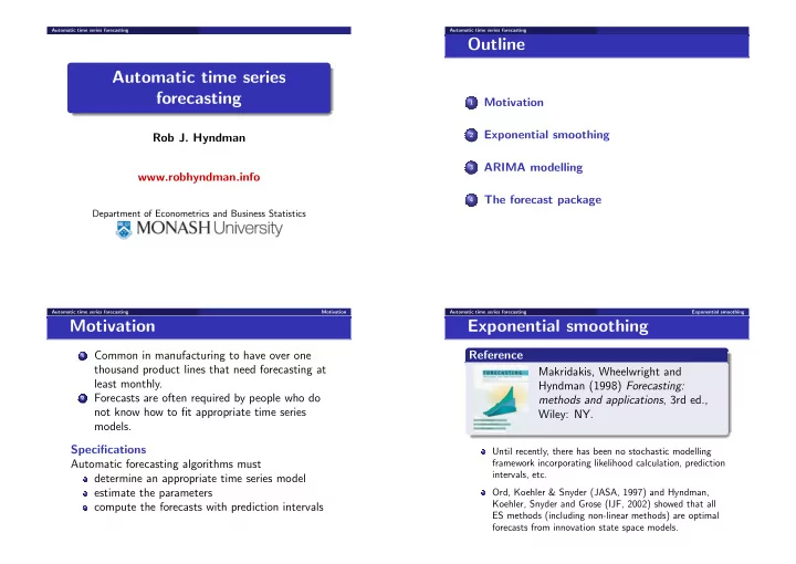
Automatic time series forecasting Automatic time series forecasting Outline Automatic time series forecasting Motivation 1 Exponential smoothing 2 Rob J. Hyndman ARIMA modelling 3 www.robhyndman.info The forecast package 4 Department of Econometrics and Business Statistics Automatic time series forecasting Motivation Automatic time series forecasting Exponential smoothing Motivation Exponential smoothing Reference Common in manufacturing to have over one 1 thousand product lines that need forecasting at Makridakis, Wheelwright and least monthly. Hyndman (1998) Forecasting: Forecasts are often required by people who do methods and applications , 3rd ed., 2 not know how to fit appropriate time series Wiley: NY. models. Specifications Until recently, there has been no stochastic modelling Automatic forecasting algorithms must framework incorporating likelihood calculation, prediction intervals, etc. determine an appropriate time series model estimate the parameters Ord, Koehler & Snyder (JASA, 1997) and Hyndman, Koehler, Snyder and Grose (IJF, 2002) showed that all compute the forecasts with prediction intervals ES methods (including non-linear methods) are optimal forecasts from innovation state space models.

Automatic time series forecasting Exponential smoothing Automatic time series forecasting Exponential smoothing Pegels’ (1969) taxonomy Automatic forecasting From Hyndman et al. (IJF, 2002): Extended by Gardner (IJF 1985), Hyndman et al. Apply each of 30 methods that are appropriate (IJF 2002), and Taylor (IJF 2003). to the data. Optimize parameters and initial Seasonal Component values using MLE (or some other criterion). Trend N A M Select best method using AIC: Component (None) (Additive) (Multiplicative) N (None) N,N N,A N,M AIC = − 2 log(Likelihood) + 2 p A (Additive) A,N A,A A,M Ad (Additive damped) Ad,N Ad,A Ad,M where p = # parameters. M (Multiplicative) M,N M,A M,M Md (Multiplicative damped) Md,N Md,A Md,M Produce forecasts using best method. General notation E T S Obtain prediction intervals using underlying ր ↑ տ state space model. Error Trend Seasonal Method performed very well in M3 competition. Automatic time series forecasting ARIMA modelling Automatic time series forecasting ARIMA modelling ARIMA modelling Automatic Algorithm Key ideas Conventional ARIMA forecasting Fit ARIMA model to y 1 , . . . , y t and forecast calculate forecasts from the best fitting y t +1 | t , . . . , y t + h | t ARIMA model Calculate out-of-sample error a t , i = ( y t + i − ˆ y t + i | t ) Calculate average Not necessarily the best forecasting ARIMA model. n − h h 1 � a 2 t , i and MSE = 1 � MSE i = MSE i Model identification either subjective and n − h − m +1 h t = m i =1 complex, or based on information criteria Choose model based on smallest MSE i or that may not give good forecasts . smallest MSE.

Automatic time series forecasting ARIMA modelling Automatic time series forecasting ARIMA modelling Automatic Algorithm Automatic Algorithm DGP: ARIMA(0,1,1) Problem: No. of series 1000, with each length 100 Procedure involves fitting ( n − m ) D model 12 True Estimated AIC where D is the number of candidate models. AAAF 10 Using nonlinear optimization is infeasible. Average MSE 8 Solution: 6 Estimate error series and fit all models using 4 OLS regression. Kalman filter provides very fast updating of 2 coefficients for each model. 2 4 6 8 10 Algorithm involves D models passed through a Forecast Horizon Kalman filter. Automatic time series forecasting ARIMA modelling Automatic time series forecasting The forecast package Automatic Algorithm forecast package DGP: ARIMA(2,1,2) No. of series 1000, with each length 100 forecast() function True Estimated AIC Takes a time series as its main argument AAAF 30 Returns forecasts from automatic ES algorithm. Average MSE Yet to implement automatic ARIMA algorithm. 20 Also has methods for objects of arima , 10 HoltWinters and StructTS classes Calls predict() when appropriate. 0 Output as class “forecast”. 2 4 6 8 10 Forecast Horizon

Automatic time series forecasting The forecast package Automatic time series forecasting The forecast package forecast package forecast package > forecast(beer) forecast class contains Original series Point Forecast Lo 80 Hi 80 Point forecasts Sep 1995 138.2864 128.5376 148.2387 Prediction interval Oct 1995 165.8323 154.0843 177.8765 Forecasting method used Nov 1995 182.7895 170.0695 195.9814 Dec 1995 186.1633 172.5645 199.7450 Residuals and other information Jan 1996 144.6313 133.8904 155.3027 Methods applying to the forecast class: Feb 1996 137.2431 127.2945 147.7794 print Mar 1996 155.1601 143.5184 166.8024 Apr 1996 139.7544 129.1742 150.2580 plot .... summary Automatic time series forecasting The forecast package Automatic time series forecasting The forecast package forecast package forecast package Forecasts from Pegels method MMM > summary(forecast(beer)) > plot(forecast(beer)) Forecast method: Pegels method MMM 200 Model Information: Pegels method MMM Smoothing parameters: 180 alpha = 0.05 beta = 0.399 gamma = 0.05 160 phi = 1 Initial values: l = 160.5127 140 b = 0.9965 s = 0.9652 0.9152 1.0322 0.9294 0.9328 0.8479 0.8965 0.9565 0.9314 1.1176 1.2275 1.2478 120 In-sample error measures: 1991 1992 1993 1994 1995 1996 1997 ME MSE MAE MPE MAPE 0.693364420 65.159550580 6.476950267 0.001983306 0.044197349

Automatic time series forecasting The forecast package forecast package Automatic ES forecasting. Automatic ARIMA modelling using AIC. Forecasting intermittent demand data using Croston’s method Forecasting using Theta method Includes 3003 time series from M3 competition. Includes 1001 time series from M competition. Includes 90 data sets from Makridakis, Wheelwright & Hyndman (1998) Available as compiled Windows binary from http://www.robhyndman.info/Rlibrary/forecast/ Plan to upload to CRAN later this year.