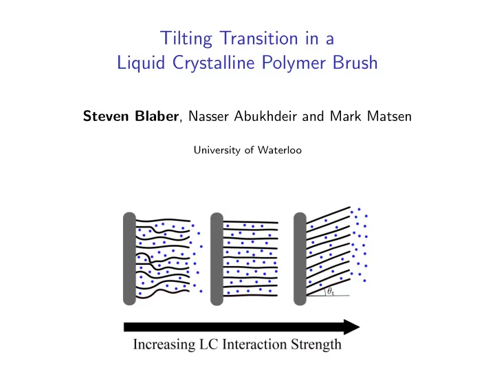
SLIDE 1
Tilting Transition in a Liquid Crystalline Polymer Brush
Steven Blaber, Nasser Abukhdeir and Mark Matsen
University of Waterloo
SLIDE 2
Motivation
SLIDE 3
Previous Work: Amoskov, Birshtein, and Pryamitsyn; Macromolecules 1996
Limitations
◮ Freely jointed chain model (no bending penalty) ◮ Director fixed along z (no tilting)
SLIDE 4
Theory
SLIDE 5 Wormlike Chain Model
Fixed contour length controlled by the degree of polymerization N and segment length b ℓc = bN . The penalty for bending in the worm-like chain model is UB = κ 2N 1 ds
ds
, with κ a dimensionless bending modulus, which controls the persistence length, ℓp = bκ .
SLIDE 6 Implicit Solvent
We will be using an implicit solvent model, which assumes a semi-dilute mixture. This corresponds to expanding the solvent entropy Ss = −
with φs = 1 − φ , assuming low polymer concentration φ ≪ 1 Ss =
2 + φ3 6 + O(φ4)
- The linear term does not effect the system and the quadratic term is
combined with the Flory-Huggins polymer-solvent interaction parameter, χ, into one parameter Λ0 with energy U0 = Λ0 2
SLIDE 7 LC Interactions
Maier-Saupe interactions: U2 = −Λ2 2
- dzdudu′φ(z, u)P2(u · u′)φ(z, u′) ,
where φ(z, u) is the concentration with orientation u and P2 is the second Legendre polynomial. Tensor order parameter: Qij(z) ≡ 3 2φ(z)
3
i & j = x, y, z = 3S(z) 2
3δij
2 (li(z)lj(z) − mi(z)mj(z)) , where S is the uniaxial and P the biaxial scalar nematic order parameters while n, l, m are orthogonal unit directors.
SLIDE 8 Self-Consistent Field Theory (SCFT)
Replace interactions on a polymer by a field, w(z, u), Ufield =
◮ Calculate φ(z, u) for a given w(z, u) ◮ Adjust w(z, u) to satisfy self-consistent equation w(z, u) = Λ0φ(z) − Λ2
This process yields the free energy F = − ln Q − 1 2
◮ Initially we assume alignment along z axis = ⇒ azimuthal symmetry, so w(z, u) → w0(z, uz) .
SLIDE 9
Results
SLIDE 10
Concentration and Scalar Order Parameter
SLIDE 11
Backfolded State: Director Fixed Along z axis
SLIDE 12 Backfolded State: Director Fixed Along z axis
Utot = 1 2
- dz
- Λ0 − Λ2S2(z)
- φ2(z) + UB
SLIDE 13 Tilted State: Director Free
Utot = 1 2
- dz
- Λ0 − Λ2S2(z)
- φ2(z) + UB
SLIDE 14 Tilted State: Director Free
Field equation β[w] ≡ w(z, u) − Λ0φ(z) + Λ2
Jacobian Jz,z′′,u,u′′ ≡ Dβ[w] Dw(z′′, u′′)
. The solution is no longer stable when an eigenvalue of the Jacobian becomes negative. The corresponding eigenvector δw(z, u) represents the change in the field that will reduce the free energy.
SLIDE 15
Tilted State: Director Free
SLIDE 16 Tilted State: Director Free
Utot = 1 2
- dz
- Λ0 − Λ2S2(z)
- φ2(z)
- Uint(z)
+UB
SLIDE 17 Tilted State: Director Free
Utot = 1 2
- dz
- Λ0 − Λ2S2(z)
- φ2(z) + UB
SLIDE 18 Phase Diagram
Utot = 1 2
- dz
- Λ0 − Λ2S2(z)
- φ2(z) + UB
SLIDE 19 Phase Diagram
Utot = 1 2
- dz
- Λ0 − Λ2S2(z)
- φ2(z) + UB
SLIDE 20 Phase Diagram
Utot = 1 2
- dz
- Λ0 − Λ2S2(z)
- φ2(z) + UB
SLIDE 21 Tilt Angle
Utot = 1 2
SLIDE 22 Tilt Angle
Ss =
2 + φ3 6 + O(φ4)
SLIDE 23 Tilt Angle
Utot =
1 2
3 φ3(z)
SLIDE 24
Conclusion
◮ Strong LC interactions can nematically collapse a polymer brush; however, it does so by tilting rather than backfolding. ◮ The transition is an instability within the implicit solvent model and is continuous once you add higher order corrections.
SLIDE 25
Future Work
◮ Use an explicit solvent model to determine the tilt angle as a function of Λ2. ◮ A strongly stretched LCP brush, swollen with either a melt of LCs or LCPs could induce local orientational order in the melt at the interface which has potential applications for LC displays.