THE COST OF REPAIRS Gabriele Puppis LaBRI / CNRS based on joint - PowerPoint PPT Presentation
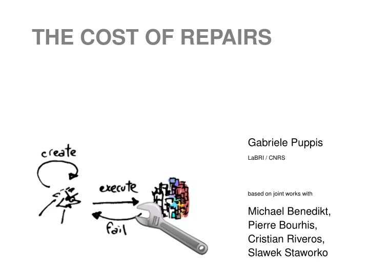
THE COST OF REPAIRS Gabriele Puppis LaBRI / CNRS based on joint works with Michael Benedikt, Pierre Bourhis, Cristian Riveros, Slawek Staworko What do you do when a computational object fails a specification? 5 Source 10000 X Target
THE COST OF REPAIRS Gabriele Puppis LaBRI / CNRS based on joint works with Michael Benedikt, Pierre Bourhis, Cristian Riveros, Slawek Staworko
What do you do when a computational object fails a specification? 5 Source 10000 X Target 1000 1050 10000 10050 100000 100050 . . . . . .
What do you do when a computational object fails a specification? 5 Source 10000 X Target 1000 1050 10000 10050 100000 100050 . . . . . . Worst-case cost of repairing source into target: t ∈ T dist ( s,t ) max s ∈ S min
What do you do when a computational object fails a specification? 5 Source 10000 X Target 1000 1050 10000 10050 100000 100050 . . . . . . Worst-case cost of repairing source into target: t ∈ T dist ( s,t ) max s ∈ S min Depends on distance (e.g., Levenstein distance)
What do you do when a computational object fails a specification? 1 1 Source 100000 X X Target 1000 1010 100000 101010 10000000 10101010 . . . . . . Worst-case cost of repairing source into target: t ∈ T dist ( s,t ) max s ∈ S min Depends on distance (e.g., Levenstein distance) Can be infinite !
Plan A. Bounded repairability of regular word languages 1) characterization 2) streaming setting 3) complexity B. Bounded repairability of regular tree languages 1) curry encodings, stepwise automata, contexts 2) characterization 3) complexity
Part A. Problem setting: Given two languages S ⊆ Σ ∗ and T ⊆ ∆ ∗ (represented by finite state automata) Decide whether max s ∈ S min t ∈ T dist ( s,t ) is finite.
Part A. Problem setting: Given two languages S ⊆ Σ ∗ and T ⊆ ∆ ∗ (represented by finite state automata) Decide whether max s ∈ S min t ∈ T dist ( s,t ) is finite. Examples 10 ∗ is bounded repairable into 10 ∗ 50 10 ∗ is not bounded repairable into ( 10 ) ∗ ( 1 + 0 ) ∗ is not bounded repairable into ( 1 + 0 ∗ 5 ) ∗
If you need to edit, Rule of thumb: you’d better do it outside a loop! Target automaton Source automaton 1 1 X Y 0 0 0 0 1 1 0 0 0 0 0 0 5 1 1
If you need to edit, Rule of thumb: you’d better do it outside a loop! Target automaton Source automaton 1 1 X Y 0 0 0 0 1 1 0 0 0 0 0 0 5 1 1
If you need to edit, Rule of thumb: you’d better do it outside a loop! Target automaton Source automaton 1 1 X Y 0 0 0 0 1 1 0 0 0 0 0 0 5 1 1 For any strategy that repairs traces of X into traces of Y: 1. either traces ( X ) ⊆ traces ( Y ) 2. or the strategy has unbounded cost.
Characterization of bounded repairability of word languages S is repairable into T with uniformly bounded cost ⇕ Given some (trimmed) automata for S and T and the DAGs of strongly connected components... Target DAG Source DAG
Characterization of bounded repairability of word languages S is repairable into T with uniformly bounded cost ⇕ Given some (trimmed) automata for S and T and the DAGs of strongly connected components... Target DAG Source DAG ...every chain of components in the source is covered by a chain of components in the target.
Characterization of bounded repairability of word languages S is repairable into T with uniformly bounded cost ⇕ Given some (trimmed) automata for S and T and the DAGs of strongly connected components... Target DAG Source DAG ...every chain of components in the source is covered by a chain of components in the target.
An example All chains of source DAG are covered by chains of target DAG ⇒ S is repairable into T with uniformly bounded cost. S = 30 ∗ 1 ∗ + 30 ∗ 2 ∗ T = 10 ∗ 1 ∗ + 20 ∗ 2 ∗ 0 2 0 3 2 2 2 2 1 1 1 0 1 1
An example All chains of source DAG are covered by chains of target DAG ⇒ S is repairable into T with uniformly bounded cost. S = 30 ∗ 1 ∗ + 30 ∗ 2 ∗ T = 10 ∗ 1 ∗ + 20 ∗ 2 ∗ 0 2 0 3 2 2 2 2 1 1 1 0 1 1
An example All chains of source DAG are covered by chains of target DAG ⇒ S is repairable into T with uniformly bounded cost. S = 30 ∗ 1 ∗ + 30 ∗ 2 ∗ T = 10 ∗ 1 ∗ + 20 ∗ 2 ∗ 0 2 0 3 2 2 2 2 1 1 1 0 1 1
An example All chains of source DAG are covered by chains of target DAG ⇒ S is repairable into T with uniformly bounded cost. S = 30 ∗ 1 ∗ + 30 ∗ 2 ∗ T = 10 ∗ 1 ∗ + 20 ∗ 2 ∗ 0 2 0 3 2 2 2 2 1 1 1 0 1 1 There is no covering relation compatible with prefixes ⇒ the repair strategy is not streaming (i.e. implementable by a sequential transducer)
An example All chains of source DAG are covered by chains of target DAG ⇒ S is repairable into T with uniformly bounded cost. S = 30 ∗ 1 ∗ + 30 ∗ 2 ∗ T = 10 ∗ 1 ∗ + 20 ∗ 2 ∗ 0 2 0 3 2 2 2 2 1 1 1 0 1 1 There is no covering relation compatible with prefixes ⇒ the repair strategy is not streaming (i.e. implementable by a sequential transducer)
Complexity of non-streaming bounded repairability problem: fixed DFA NFA fixed CONST P PSPACE DFA P coNP PSPACE NFA PTIME coNP PSPACE
Complexity of non-streaming bounded repairability problem: fixed DFA NFA fixed CONST P PSPACE DFA P coNP PSPACE NFA PTIME coNP PSPACE Complexity of streaming bounded repairability problem: fixed DFA NFA fixed CONST P PSPACE DFA P P PSPACE ≤ PSPACE ≤ PSPACE ≤ EXP NFA ≥ P ≥ P ≥ PSPACE
Part B. New tools for a more general setting... Languages of words: Languages of unranked trees: insersions / deletions insertions / deletions finite state automata stepwise tree automata components & traces components & contexts coverability of chains coverability of synopsis trees
Edit operations on unranked trees: deletions ⋮ X ... ... ... ... ... ... ... ... ...
Edit operations on unranked trees: deletions ⋮ ... ... ... ... ... ... ... ... ...
Edit operations on unranked trees: insertions ⋮ + ... ... ... ... ... ... ... ... ...
Edit operations on unranked trees: insertions ⋮ ... ... ... ... ... ... ... ... ...
An example Target Source r r c ... c a ... a e d a ... a b ... b b ... b c ... c
An example Target Source r r c ... c a ... a e d a ... a b ... b b ... b c ... c r c ... c X d a ... a b ... b
An example Target Source r r c ... c a ... a e d a ... a b ... b b ... b c ... c r + c ... c a ... a b ... b
An example Target Source r r c ... c a ... a e d a ... a b ... b b ... b c ... c r e c ... c a ... a b ... b
Bottom-up automata on ranked (binary) trees: ... δ ( q 1 ,q 2 ) q 1 q 2 How to parse unranked trees?
Bottom-up automata on ranked (binary) trees: ... δ ( q 1 ,q 2 ) q 1 q 2 How to parse unranked trees? Encode them using binary trees!
The curry encoding @ ... 0 n ≅ @ ... n @ 2 1 2 0 1 @ 0 0 @ 1 1 @ ... 2 2 n ⋮ n
The curry encoding @ ... 0 n ≅ @ ... n @ 2 1 2 0 1 @ 0 0 @ 1 1 @ ... 2 2 n ⋮ n
The curry encoding @ ... 0 n ≅ @ ... n @ 2 1 2 0 1 @ 0 0 @ 1 1 @ ... 2 2 n ⋮ n
The curry encoding @ ... 0 n ≅ @ ... n @ 2 1 2 0 1 @ 0 ≅ 0 @ 1 1 @ ... 2 2 n ⋮ n
The curry encoding @ ... 0 n ≅ @ ... n @ 2 1 2 0 1 @ 0 ≅ 0 @ 1 1 @ ... 2 2 n ⋮ n Stepwise automata = bottom-up on curry encodings
An example q final r @ ≅ a ... a b @ @ . . . . . . ⋮ a b @ @ b r a c b c q r q a q c
An example q final r @ ≅ a ... a b @ @ . . . . . . ⋮ a b @ @ b r a c b c q r q a q c r ↦ q r q r @ q a ↦ q r a ↦ q a ↦ q b @ q c q c ↦ b q b q r @ q c ↦ q final c ↦ q c
An example q final r @ ≅ a ... a b @ @ . . . . . . ⋮ a b q a q b @ @ b r a c b c q r q a q b q c r ↦ q r q r @ q a ↦ q r a ↦ q a ↦ q b @ q c q c ↦ b q b q r @ q c ↦ q final c ↦ q c
An example q final r @ ≅ q r q c a ... a b @ @ . . . . . . . . . . . . ⋮ a b q r q c q a q b @ @ b r a c b c q r q a q b q c r ↦ q r q r @ q a ↦ q r a ↦ q a ↦ q b @ q c q c ↦ b q b q r @ q c ↦ q final c ↦ q c
An example q final r @ ≅ q r q c a ... a b @ @ . . . . . . . . . . . . ⋮ a b q r q c q a q b @ @ b r a c b c q r q a q b q c r ↦ q r q r @ q a ↦ q r a ↦ q a ↦ q b @ q c q c ↦ b q b q r @ q c ↦ q final c ↦ q c
Contexts = trees with holes @ ... ? n ≅ @ ... n @ 2 1 2 1 ? @ 0 ≅ 0 @ ? ? @ ... 2 2 n ⋮ n
Contexts = trees with holes @ ... ? ? n ≅ @ ... n @ 2 1 2 1 ? ? @ 0 ≅ 0 @ ? ? ? ? @ ... 2 2 n ⋮ n
Contexts = trees with holes @ ... ? ? n ≅ @ ... n @ 2 1 2 1 ? ? @ 0 ≅ 0 @ ? ? ? ? @ ... 2 2 n ⋮ n C � → q Contexts can be parsed between two states: p (accessibility of states and components are defined accordingly)
Recall: a run of a finite state automaton induces a chain of components ... Likewise, a run of a stepwise automaton induces a synopsis tree (i.e. a tree of components).
Recommend
More recommend
Explore More Topics
Stay informed with curated content and fresh updates.


