
SLIDE 1
“Telescope of Theory”: Radiative Transfer Studies of a Young Star Forming Object
- M. Yamada(ASIAA)、M.N. Machida(NAOJ)、
- S. Inutsuka(Nagoya-U.), K. Tomisaka、Y. Kurono(NAOJ)
1
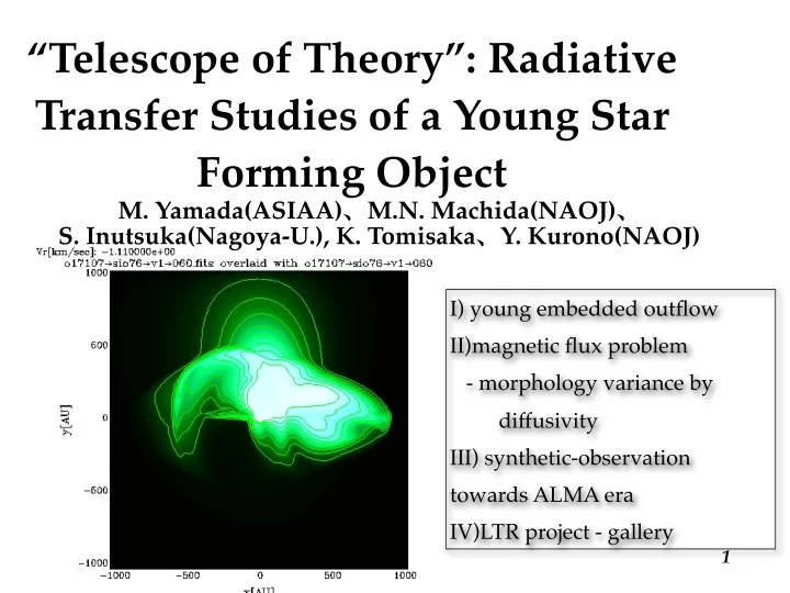
I) young embedded outflow II)magnetic flux problem
- morphology variance by
diffusivity III) synthetic-observation towards ALMA era IV)LTR project - gallery