
SLIDE 1
UniOS-FB9-IMU-BWL/MSWI-Rieger-SS06-WiKyb-05: System Dynamics Basics (Delays) (1 / 8)
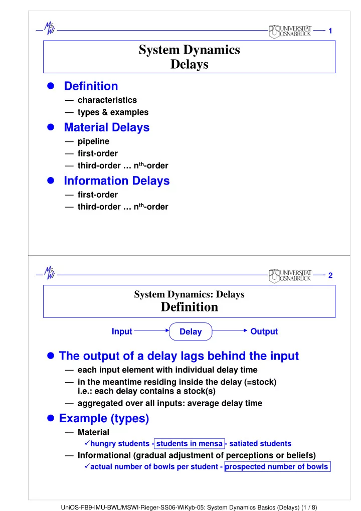
System Dynamics Delays Definition characteristics types & - - PDF document
1 System Dynamics Delays Definition characteristics types & examples Material Delays pipeline first-order third-order n th -order Information Delays first-order third-order n th -order 2 System
UniOS-FB9-IMU-BWL/MSWI-Rieger-SS06-WiKyb-05: System Dynamics Basics (Delays) (1 / 8)
UniOS-FB9-IMU-BWL/MSWI-Rieger-SS06-WiKyb-05: System Dynamics Basics (Delays) (2 / 8)
1 0.75 0.5 0.25 2 4 6 8 10 12 14 16 18 20 22 24 Time (Hour) hungry students : Current
2 1.5 1 0.5 11 12 13 14 15 16 Time (Hour) hungry : Current % satiated : Current % eating : Current %
UniOS-FB9-IMU-BWL/MSWI-Rieger-SS06-WiKyb-05: System Dynamics Basics (Delays) (3 / 8)
2 1.5 1 0.5 11 12 13 14 15 16 Time (Hour) hungry : Current % satiated : Current % wait and eat : Current %
Model equations: average eating time=1 hungry=PULSE(12, 0.01)/0.01 wait and eat= INTEG (hungry-satiated,0) satiated=wait and eat/average eating time
satiated=DELAY1I(hungry, average eating time, 0) TIME STEP=0.01
Model equations: average eating time=1 hungry=PULSE(12, 0.01)/0.01 waiting= INTEG (hungry-served,0) served=waiting/(average eating time/2) eating= INTEG (served-satiated,0) satiated=eating/(average eating time/2) TIME STEP=0.01
2 1.5 1 0.5 11 12 13 14 15 16 Time (Hour)
hungry : Current % satiated : Current % waiting : Current % eating : Current %
UniOS-FB9-IMU-BWL/MSWI-Rieger-SS06-WiKyb-05: System Dynamics Basics (Delays) (4 / 8)
Model equations: average eating time=1 hungry=PULSE(12, 0.01)/0.01 waiting= INTEG (hungry-served,0) served=waiting/(average eating time/3) paying= INTEG (served-paid,0) paid=paying/(average eating time/3) eating= INTEG (paid-satiated,0) satiated=eating/(average eating time/3)
satiated=DELAY3I(hungry, average eating time, 0) TIME STEP=0.01
2 1.5 1 0.5 11 12 13 14 15 16 Time (Hour)
hungry : Current % satiated : Current % waiting : Current % paying : Current % eating : Current %
9th-order material delay
2 1.5 1 0.5 11 12 13 14 15 16 Time (Hour)
hungry : Current % satiated : Current % waiting : Current % paying : Current % eating : Current %
Model equations: average eating time=1 hungry=PULSE(12, 0.01)/0.01 waiting= INTEG (hungry-served,0) served=DELAY3I(hungry, average eating time/3, 0) paying= INTEG (served-paid,0) paid=DELAY3I(served, average eating time/3, 0) eating= INTEG (paid-satiated,0) satiated=DELAY3I(paid, average eating time/3, 0) TIME STEP=0.01
UniOS-FB9-IMU-BWL/MSWI-Rieger-SS06-WiKyb-05: System Dynamics Basics (Delays) (5 / 8)
hungry : Current % satiated0 : Current % satiated1 : Current % satiated3 : Current % satiated9 : Current %
UniOS-FB9-IMU-BWL/MSWI-Rieger-SS06-WiKyb-05: System Dynamics Basics (Delays) (6 / 8)
Model Equations: additional beginners=0 avg time of studies=9 beginners=500+STEP(additional beginners, 10) graduates=DELAY3(beginners, avg time of studies) … (s.left below) …
1,000 6,000 500 3,000 10 20 30 40 50 60 70 80 90 100 Time (Month)
beginners : add100 graduates : add100 students : add100 students : init0
students= INTEG (+beginners-graduates, beginners*avg time of studies)
students= INTEG (+beginners-graduates, 0)
200 170 140 110 80 5 10 15 20 25 30 35 40 45 50 Time (Month) Actual Value : Current Perception : Current
Model equations: Actual Value=100+STEP(50, 5) Adjustment=Gap/Adjustment Time Adjustment Time=6 Gap=Actual Value-Perception Perception= INTEG (Adjustment,Actual Value)
Perception=SMOOTH(Actual Value, Adjustment Time)
UniOS-FB9-IMU-BWL/MSWI-Rieger-SS06-WiKyb-05: System Dynamics Basics (Delays) (7 / 8)
63% 86% 95%
UniOS-FB9-IMU-BWL/MSWI-Rieger-SS06-WiKyb-05: System Dynamics Basics (Delays) (8 / 8)
Vergleich Delay1 und Delay3
200 175 150 125 100 3 6 9 12 15 18 Time (Month) Zuflußrate - BASIS Abflußrate Delay1 - BASIS Abflußrate Delay3 - BASIS Pipe line Abfluß rate Delay3 RT2 Delay 3 RT1 Delay 3 LV3 Delay3 LV2 Delay3 LV1 Delay3 Abfluß rate3 Abfluß rate1 Verzögerungszeit Abfluß rate Delay1 Zufluß rate LV Delay1
SMOOTH3: Die Glättung 1. bis 3. Ordnung
200 175 150 125 100 3 6 9 12 15 18 Time (Month)
Input - BASIS LV1S3 - BASIS LV2S3 - BASIS LV3S3 - BASIS Output Smooth3 - BASIS
RT2 S3 RT1 S3 Input RT3 S3 Glättungs faktor LV3S3 LV2S3 LV1S3 Output Smooth 3 Output Smooth Delta Smooth LV Smooth Verzögerungszeit