
SLIDE 1
Symmetries of stochastic colored vertex models
Pavel Galashin (UCLA) Dimers in Combinatorics and Cluster Algebras 2020 arXiv:2003.06330
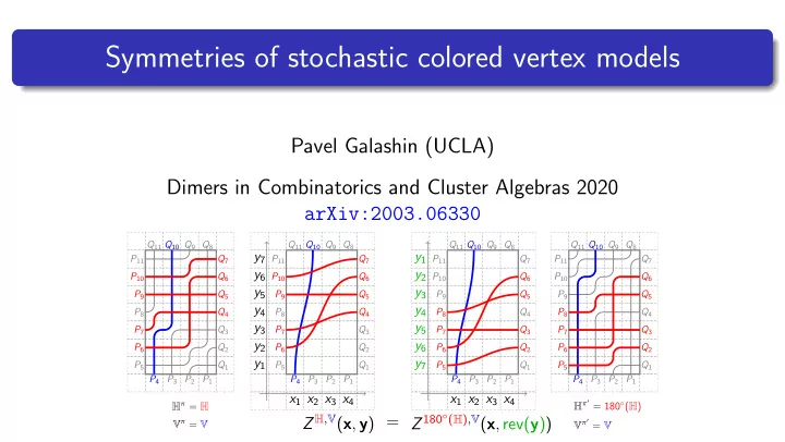
P1 P2 P3 P4 P5 P6 P7 P8 P9 P10 P11 Q1 Q2 Q3 Q4 Q5 Q6 Q7 Q8 Q9 Q10 Q11 P1 P2 P3 P4 P5 P6 P7 P8 P9 P10 P11 Q1 Q2 Q3 Q4 Q5 Q6 Q7 Q8 Q9 Q10 Q11
x1 x2 x3 x4 y1 y2 y3 y4 y5 y6 y7
P1 P2 P3 P4 P5 P6 P7 P8 P9 P10 P11 Q1 Q2 Q3 Q4 Q5 Q6 Q7 Q8 Q9 Q10 Q11
x1 x2 x3 x4 y7 y6 y5 y4 y3 y2 y1
P1 P2 P3 P4 P5 P6 P7 P8 P9 P10 P11 Q1 Q2 Q3 Q4 Q5 Q6 Q7 Q8 Q9 Q10 Q11 Hπ = H Vπ = V
= Z H,V(x, y) Z 180◦(H),V(x, rev(y))
Hπ′ = 180◦(H) Vπ′ = V