1 Curve sketching Symmetries, envelopes and square roots 1.5 - - PowerPoint PPT Presentation

1 Curve sketching — Symmetries, envelopes and square roots

1.5 Comments on symmetries.

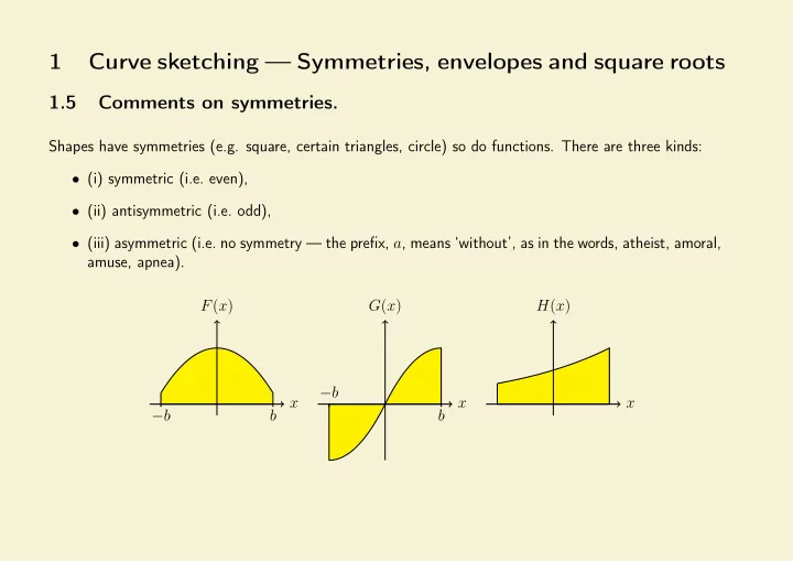
Shapes have symmetries (e.g. square, certain triangles, circle) so do functions. There are three kinds:

• (i) symmetric (i.e. even),
• (ii) antisymmetric (i.e. odd),
• (iii) asymmetric (i.e. no symmetry — the prefix, a, means ‘without’, as in the words, atheist, amoral,

amuse, apnea). −b b x F(x) −b b x G(x) x H(x)

−b b x F(x) −b b x G(x) x H(x) Examples of even functions: x2, x4, cos x, e−x2, sin2 x, x3 sin x, cosh x, f(x) + f(−x). Examples of odd functions: x, x3, sin x, xe−x2, x cos x, sinh x, f(x) − f(−x). Examples of asymmetric functions: ex, sin(x + 1

4π),

x + |x|. Note: We have the following “multiplication tables” for symmetries: even × even = even

• dd × odd = even

even × odd = odd This is just like the addition of even and odd numbers....

1.6 Envelopes.

This involves the product of two functions, one of which oscillates. We will look in detail at the functions, x cos x, x sin x, (cos x)/x and e−|x| sin 100x.

• Black disks mark where sin x = 0, i.e. where x = nπ.
• Here f(x) is positive, and since −1 ≤ sin x ≤ 1, then,

−f(x) ≤ f(x) sin x ≤ f(x).

• It’s a little more complicated when f(x) has zeroes.

General strategy:

• Check for symmetries.
• Draw both f(x) and −f(x) first.
• Mark where the sinusoid is zero. Likewise for f(x),
• Finally attempt to sketch the curve.

x x cos x Figure 1.26

• We first mark in the functions x and −x as the dashed lines, and therefore we know that x cos x

must lie between these two extremes.

• The zeros of cos x are at x = ±π/2, ±3π/2 and so on, so these are marked by black disks on the

x-axis.

• Another zero arises at x = 0 due to the factor, x, in x cos x.
• Finally, we note that the function is odd (odd×even). (Useful to state if your diagram doesn’t make

it obvious!)

Figure 1.27 x x sin x

• This example is very similar to that shown in Figute 1.26. But it has a sine rather than a cosine.
• The function is even because x sin x is odd×odd.
• sin x has single zeros at 0, ±π, ±2π, ±3π and so on.
• There is a second zero at x = 0 because both the factors in x sin x have simple zeros.
• Therefore there is a double zero at x = 0 and the curve will look like a parabola near there.

Figure 1.28 x (cos x)/x

• We first mark in the functions 1/x and −1/x.
• These tend to ±∞ as x → 0.
• Note that both cos x and x are positive when x is slightly greater than zero.
• An odd function. The zeros of cos x are at odd multiples of 1

2π.

Figure 1.29 x e−|x| sin 100x

• The function e−|x| decays exponentially as x → ±∞. It is even.
• The envelope, ±e−|x|, has been sketched.
• The odd function sin 100x oscillates very quickly (the period is π/50).
• e−|x| sin 100x is an odd function.
• This is an example of an AM (Amplitude Modulation) radio signal: the carrier wave (sin 100x) has

its amplitude modulated by the signal, e−|x|.

1.7 Square roots of functions.

• A little bit of care needs to be taken whenever one needs to sketch the square root of a function.
• Both roots? Often resolved when considering the application.
• But what happens when one takes the square root of a function which has a single zero?

Figure 1.30 Yes — a vertical tangent!

x y = √ 1 − x2 Figure 1.31. x y where y2 = 1 − x2 I am simply making the distinction between writing y = √ 1 − x2 explicitly, and writing y2 = 1 − x2 in terms of what one plots. In the right hand graph the negative values of y are allowed, whereas they are not allowed on the left. Clearly this is a circle since x2 + y2 = 1. But what is happening near x = 1 in this case?

x y where y2 = 1 − x2 Clearly there is a vertical tangent at x = 1, but is it the square root of a linear factor? Just consider the positive root: y = √ 1 − x2 ⇒ y =

• (1 + x)(1 − x).

When x 1 then (1 + x) ≃ 2 and therefore the equation becomes y =

• (1 + x)(1 − x) ≃
• 2(1 − x).

This is the square root of a linear factor, just as in Figure 1.30.

x y = (x − 2)(x − 1)(x + 1)(x + 2) Figure 1.9 Figure 1.32 x y =

• (x − 2)(x − 1)(x + 1)(x + 2)
• We have y = (x − 2)(x − 1)(x + 1)(x + 2) on the left and y =
• (x − 2)(x − 1)(x + 1)(x + 2) on

the right.

• The dotted lines on the right denote the extra curves for y2 = (x − 2)(x − 1)(x + 1)(x + 2), i.e. for

y = ±

• (x − 2)(x − 1)(x + 1)(x + 2).
• At the roots, x = ±1, ±2 we have vertical tangents.

1.8 Ratios of polynomials.

Sounds scary but it’s systematic. An example: y = (x − 1)2(x + 2) x(x − 3)2 . First we collect basic information of the following kind:

• the locations of all zeros and their multiplicity (i.e. single, double and so on);
• the locations of all poles (i.e. infinities) which are the zeros of the denominator, and we also need

their multiplicity;

• the large-x behaviour.

For the above example we have the following: Zeros at x = 1, 1, −2 i.e. x = 1 twice and x = −2 once, Infinities at x = 0, 3, 3 i.e. x = 3 twice and x = 0 once, y → 1 as x → ±∞. When x ≫ 1 then y ≃ x3 x3 = 1.

A straightforward case of a pole at x = 0. As x increases past x = 0, the sign of y changes, but y will have descended down to −∞ before re-emerging at +∞. This infinite discontinuity always happens at a single pole. Figure 1.33. x y = 1/x As Figure 1.33 but the pole is now at x = 1. Figure 1.34. x y = 1/(x − 1)

This is a double pole at x = 1. I have indicated the location of the double pole by a pair of dashed lines. As x increases through x = 1, then (x − 1)2 doesn’t change sign. Hence the curve ascends to +∞ and then returns from +∞. Figure 1.35. x y = 1/(x − 1)2 This is a triple pole at x = 1, the pres- ence of which is indicated by three dashed

• lines. The fact that it is a cube means

that there will be a sign change as x in- creases past x = 1. So this looks very similar to the single pole case. Figure 1.36. x y = 1/(x − 1)3

x Figure 1.37 y = 1 x2 − 1

• There are no zeros.
• Poles at x = −1 and x = 1 because x2 − 1 = (x − 1)(x + 1).
• When x → ±∞ then y → 0+.

Refer to full notes for the details of the joining of the dots! All of our examples will follow a similar logic. The behaviour of the curve will then depend on the multiplicity of the zeros and poles.

x y = x x2 − 1 Figure 1.38

• Zero at x = 0.
• Poles at x = −1 and x = 1.
• When x → ∞ then y → 0+.
• When x → −∞ then y → 0−.

It is worth comparing Figures 1.37 and 1.38 to see the difference caused by the addition of a zero.

y = x(x − 1) (x + 1)(x − 2). Zeros at x = 0, 1. Poles at x = −1, 2. When x → ±∞ then y → 1. Similar logic to the previous example. Figure 1.39. x y y = x(x − 1)2 (x + 1)2(x − 2). Zeros at x = 0, 1, 1. Poles at x = −1, −1, 2. When x → ±∞ then y → 1. Figure 1.40. x y

y = x(x − 1)2 (x + 1)(x − 2) Zeros at x = 0, 1, 1. Poles at x = −1, 2. When x → ±∞ then y ∼ x. Figure 1.41. x y A slightly modified version of both Figures 1.39 and 1.40. Note the different large-x behaviour here. Final note: it is possible to go a little further with the large-|x| behaviour and find that, y = x(x − 1)2 (x + 1)(x − 2) = x − 1 + 2x − 2 x2 − x − 2, but I shall not be covering this extra analysis.