1 Whered Ya Get Them P( )? Its Like Having Twins is the - - PDF document

1
SMART_READER_LITE
LIVE PREVIEW

1 Whered Ya Get Them P( )? Its Like Having Twins is the - - PDF document

Two Envelopes Revisited Subjectivity of Probability The two envelopes problem set -up Belief about contents of envelopes Since implied distribution over X is not a true probability Two envelopes: one contains $X, other


slide-1
SLIDE 1

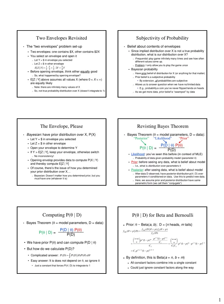
1 Two Envelopes Revisited

  • The “two envelopes” problem set-up
  • Two envelopes: one contains $X, other contains $2X
  • You select an envelope and open it
  • Let Y = $ in envelope you selected
  • Let Z = $ in other envelope
  • Before opening envelope, think either equally good
  • So, what happened by opening envelope?
  • E[Z | Y] above assumes all values X (where 0 < X < )

are equally likely

  • Note: there are infinitely many values of X
  • So, not true probability distribution over X (doesn’t integrate to 1)

Y Y Y Z E

Y 4 5 2 1 2 2 1

2 ] | [     

Subjectivity of Probability

  • Belief about contents of envelopes
  • Since implied distribution over X is not a true probability

distribution, what is our distribution over X?

  • Frequentist: play game infinitely many times and see how often

different values come up.

  • Problem: I only allow you to play the game once
  • Bayesian probability
  • Have prior belief of distribution for X (or anything for that matter)
  • Prior belief is a subjective probability
  • By extension, all probabilities are subjective
  • Allows us to answer question when we have no/limited data
  • E.g., probability a coin you’ve never flipped lands on heads
  • As we get more data, prior belief is “swamped” by data

The Envelope, Please

  • Bayesian: have prior distribution over X, P(X)
  • Let Y = $ in envelope you selected
  • Let Z = $ in other envelope
  • Open your envelope to determine Y
  • If Y > E[Z | Y], keep your envelope, otherwise switch
  • No inconsistency!
  • Opening envelop provides data to compute P(X | Y)

and thereby compute E[Z | Y]

  • Of course, there’s the issue of how you determined

your prior distribution over X…

  • Bayesian: Doesn’t matter how you determined prior, but you

must have one (whatever it is)

Revisting Bayes Theorem

  • Bayes Theorem ( = model parameters, D = data):
  • Likelihood: you’ve seen this before (in context of MLE)
  • Probability of data given probability model (parameter )
  • Prior: before seeing any data, what is belief about model
  • I.e., what is distribution over parameters 
  • Posterior: after seeing data, what is belief about model
  • After data D observed, have posterior distribution p( | D) over

parameters  conditioned on data. Use this to predict new data.

  • Here, we assume prior and posterior distribution have same

parametric form (we call them “conjugate”)

P(D | ) P() P(D) P( | D) =

“Prior” “Likelihood” “Posterior”

Computing P(θ | D)

  • Bayes Theorem ( = model parameters, D = data):
  • We have prior P() and can compute P(D | )
  • But how do we calculate P(D)?
  • Complicated answer:
  • Easy answer: It is does not depend on , so ignore it
  • Just a constant that forces P( | D) to integrate to 1

P(D | ) P() P(D) P( | D) =

    d P D P D P ) ( ) | ( ) (

P(θ | D) for Beta and Bernoulli

 Prior:  ~ Beta(a, b); D = {n heads, m tails}  By definition, this is Beta(a + n, b + m)  All constant factors combine into a single constant  Could just ignore constant factors along the way

) ( ) ( ) | ( ) | (

| |

D f p f p D f D p f

D D D

      

   1 1 3

) 1 (

   

 

b m a n

p p C

1 1 2 1 2 1 1 1

) 1 ( ) 1 ( ) 1 ( ) 1 (

   

                   

 

b a m n b a m n

p p p p C C C C p p p p

n m n n m n

slide-2
SLIDE 2

2 Where’d Ya Get Them P()?

  is the probability a coin turns up heads  Model  with 2 different priors:  P1() is Beta(3,8) (blue)  P2() is Beta(7,4) (red)  They look pretty different!  Now flip 100 coins; get 58 heads and 42 tails  What do posteriors look like?

It’s Like Having Twins

 As long as we collect enough data, posteriors will

converge to the correct value!

From MLE to Maximum A Posteriori

  • Recall Maximum Likelihood Estimator (MLE) of 
  • Maximum A Posteriori (MAP) estimator of :

where g() is prior distribution of .

  • As before, can often be more convenient to use log:
  • MAP estimate is the mode of the posterior distribution

n i i MLE

X f

1

) | ( max arg  

) ,..., , ( ) ( ) | ,..., , ( max arg ) ,..., , | ( max arg

2 1 2 1 2 1 n n n MAP

X X X h g X X X f X X X f    

 

         

 n i i MAP

X f g

1

)) | ( log( )) ( log( max arg   

) | ( ) ( max arg ) ,..., , ( ) ( ) | ( max arg

1 2 1 1

 

 

         

n i i n n i i

X f g X X X h g X f    

 

Conjugate Distributions Without Tears

  • Just for review…
  • Have coin with unknown probability  of heads
  • Our prior (subjective) belief is that  ~ Beta(a, b)
  • Now flip coin k = n + m times, getting n heads, m tails
  • Posterior density: ( | n heads, m tails)~Beta(a+n,b+\m)
  • Beta is conjugate for Bernoulli, Binomial, Geometric, and

Negative Binomial

  • a and b are called “hyperparameters”
  • Saw (a + b – 2) imaginary trials, of those (a – 1) are “successes”
  • For a coin you never flipped before, use Beta(x, x) to

denote you think coin likely to be fair

  • How strongly you feel coin is fair is a function of x

Mo’ Beta Multinomial is Multiple Times the Fun

  • Dirichlet(a1, a2, ..., am) distribution
  • Conjugate for Multinomial
  • Dirichlet generalizes Beta in same way Multinomial generalizes

Bernoulli/Binomial

  • Intuitive understanding of hyperparameters:
  • Saw imaginary trials, with (ai – 1) of outcome i
  • Updating to get the posterior distribution
  • After observing n1 + n2 + ... + nm, new trials with ni of outcome i...
  • ... posterior distribution is Dirichlet(a1+ n1, a2 + n2, ..., am + nm)

m ai 

 m i 1

 

n i a i n n

i

x a a a B x x x f

1 1 2 1 2 1

) ,..., , ( 1 ) ,..., , (

slide-3
SLIDE 3

3 Best Short Film in the Dirichlet Category

  • And now a cool animation of Dirichlet(a, a, a)
  • This is actually log density (but you get the idea…)

Thanks Wikipedia!

Getting Back to your Happy Laplace

  • Recall example of 6-sides die rolls:
  • X ~ Multinomial(p1, p2, p3, p4, p5, p6)
  • Roll n = 12 times
  • Result: 3 ones, 2 twos, 0 threes, 3 fours, 1 fives, 3 sixes
  • MLE: p1=3/12, p2=2/12, p3=0/12, p4=3/12, p5=1/12, p6=3/12
  • Dirichlet prior allows us to pretend we saw each
  • utcome k times before. MAP estimate:
  • Laplace’s “law of succession”: idea above with k = 1
  • Laplace estimate:
  • Laplace: p1=4/18, p2=3/18, p3=1/18, p4=4/18, p5=2/18, p6=4/18
  • No longer have 0 probability of rolling a three!

mk n k X p

i i

   m n X p

i i

   1

Good Times With Gamma

  • Gamma(a, l) distribution
  • Conjugate for Poisson
  • Also conjugate for Exponential, but we won’t delve into that
  • Intuitive understanding of hyperparameters:
  • Saw a total imaginary events during l prior time periods
  • Updating to get the posterior distribution
  • After observing n events during next k time periods...
  • ... posterior distribution is Gamma(a + n, l + k)
  • Example: Gamma(10, 5)
  • Saw 10 events in 5 time periods. Like observing at rate = 2
  • Now see 11 events in next 2 time periods  Gamma(21, 7)
  • Equivalent to updated rate = 3

It’s Normal to Be Normal

  • Normal(m0, s0

2) distribution

  • Conjugate for Normal (with unknown m, known s2)
  • Intuitive understanding of hyperparameters:
  • A priori, believe true m distributed ~ N(m0, s02)
  • Updating to get the posterior distribution
  • After observing n data points...
  • ... posterior distribution is:

                                  

 

1 2 2 2 2 2 1 2

1 , 1 s s s s s s m n n x N

n i i