Survival Analysis http://www.isrec.isb-sib.ch/~darlene/EMBnet/ - - PDF document

1

EMBnet Course – Introduction to Statistics for Biologists 23 Jan 2009

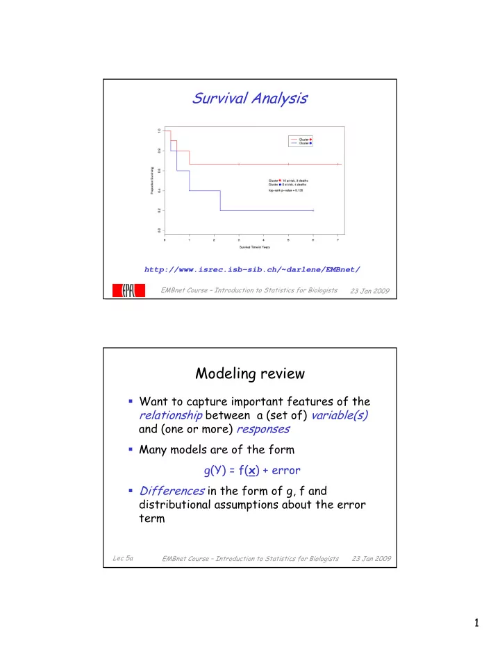
Survival Analysis

http://www.isrec.isb-sib.ch/~darlene/EMBnet/

EMBnet Course – Introduction to Statistics for Biologists 23 Jan 2009 Lec 5a

Modeling review

Want to capture important features of the relationship between a (set of) variable(s) and (one or more) responses Many models are of the form g(Y) = f(x) + error Differences in the form of g, f and distributional assumptions about the error term

2

EMBnet Course – Introduction to Statistics for Biologists 23 Jan 2009 Lec 5a

Examples of Models

Linear: Y = β0 + β1x + ε Linear: Y = β0 + β1x + β2x2 + ε (Intrinsically) Nonlinear: Y = αx1βx2γ x3δ + ε Generalized Linear Model (e.g. Binomial): ln(p/[1-p]) = β0 + β1x1 + β2x2 Proportional Hazards (in Survival Analysis): h(t) = h0(t) exp(βx)

EMBnet Course – Introduction to Statistics for Biologists 23 Jan 2009 Lec 5a

Survival data

In many medical studies, an outcome of interest is the time to an event The event may be – adverse (e.g. death, tumor recurrence) – positive (e.g. leave from hospital) – neutral (e.g. use of birth control pills) Time to event data is usually referred to as survival data – even if the event of interest has nothing to do with ‘staying alive’ In engineering, often called reliability data

3

EMBnet Course – Introduction to Statistics for Biologists 23 Jan 2009 Lec 5a

Censoring

If all lifetimes were fully observed, then we have a continuous variable We have already looked at some methods for analyzing continuous variables For survival data, the event may not have

• ccurred for all study subjects during the

follow-up period Thus, for some individuals we will not know the exact lifetime, only that it exceeds some value Such incomplete observations are said to be censored

EMBnet Course – Introduction to Statistics for Biologists 23 Jan 2009 Lec 5a

Survival modeling

Response T is a (nonnegative) lifetime For most random variables we work with the cumulative distribution function (cdf) F(t) (=P(T <= t)) and the density function f(t) (=height of the histogram) For lifetime (survival) data, it’s more usual to work with the survival function S(t) = 1 – F(t) = P(T > t) and the instantaneous failure rate, or hazard function h(t) = limΔt->0P(t ≤ T< t+Δt | T ≥ t)/ Δt

4

EMBnet Course – Introduction to Statistics for Biologists 23 Jan 2009 Lec 5a

Survival function properties

The survival function S(t) = 1 – F(t) = P(T > t) is the probability that the time to event is later than some specified time Usually assume that S(0) = 1 – that is, the event is certain to occur after time 0 The survival function is nonincreasing: S(u) <= S(t) if time u > time t That is, survival is less probable as time increases S(t) → 0 as t → ∞ (no ‘eternal life’)

EMBnet Course – Introduction to Statistics for Biologists 23 Jan 2009 Lec 5a

Relations between functions

Cumulative hazard function H(t) = ∫0t h(s) ds h(t) = f(t)/S(t) H(t) = -log S(t)

5

EMBnet Course – Introduction to Statistics for Biologists 23 Jan 2009 Lec 5a

Kaplan-Meier estimator

In order to answer questions about T, we need to estimate the survival function Common to use the Kaplan-Meier (also called product limit ) estimator ‘Down staircase’, typically shown graphically When there is no censoring, the KM curve is equivalent to the empirical distribution Can test for differences between groups with the log-rank test

EMBnet Course – Introduction to Statistics for Biologists 23 Jan 2009 Lec 5a

Cox proportional hazards model

Baseline hazard function h0(t) Modified multiplicatively by covariates Hazard function for individual case is h(t) = h0(t) exp(β1x1 + β2x2 + … + βpxp) If nonproportionality: – 1. Does it matter – 2. Is it real

6

EMBnet Course – Introduction to Statistics for Biologists 23 Jan 2009 Lec 5a

Example: Survival analysis with gene expression data

Bittner et al. dataset: – 15 of the 31 melanomas had associated survival times – 3613 ‘strongly detected’ genes

EMBnet Course – Introduction to Statistics for Biologists 23 Jan 2009 Lec 5a

‘cluster’ unclustered

Average linkage hierarchical clustering

7

EMBnet Course – Introduction to Statistics for Biologists 23 Jan 2009 Lec 5a

Survival analysis: Bittner et al.

Bittner et al. also looked at differences in survival between the two groups (the ‘cluster’ and the ‘unclustered’ samples) The ‘cluster’ seemed associated with longer survival

EMBnet Course – Introduction to Statistics for Biologists 23 Jan 2009 Lec 5a

Kaplan-Meier survival curves

8

EMBnet Course – Introduction to Statistics for Biologists 23 Jan 2009 Lec 5a

unclustered cluster

Average linkage hierarchical clustering, survival samples only

EMBnet Course – Introduction to Statistics for Biologists 23 Jan 2009 Lec 5a

Kaplan-Meier survival curves, new grouping

9

EMBnet Course – Introduction to Statistics for Biologists 23 Jan 2009 Lec 5a

Identification of genes associated with survival

For each gene j, j = 1, …, 3613, model the instantaneous failure rate, or hazard function, h(t) with the Cox proportional hazards model: h(t) = h0(t) exp(βjxij) and look for genes with both : large effect size βj large standardized effect size βj/SE(βj)

^ ^ ^

EMBnet Course – Introduction to Statistics for Biologists 23 Jan 2009 Lec 5a

10

EMBnet Course – Introduction to Statistics for Biologists 23 Jan 2009 Lec 5a

Advantages of modeling

Can address questions of interest directly – Contrast with the indirect approach: clustering, followed by tests of association between cluster group and variables of interest Great deal of existing machinery Quantitatively assess strength of evidence

EMBnet Course – Introduction to Statistics for Biologists 23 Jan 2009 Lec 5a

Survival analysis in R

R package survival A survival object is made with the function Surv() What you have to tell Surv – time : observed survival time – event : indicator saying whether the event

• ccurred (event=TRUE) or is censored

(event=FALSE) Analyze with Kaplan-Meier curve: survfit, log-rank test: survdiff Cox proportional hazards model: coxph