Summary on transport code descriptions Remarks on the nature of - - PowerPoint PPT Presentation

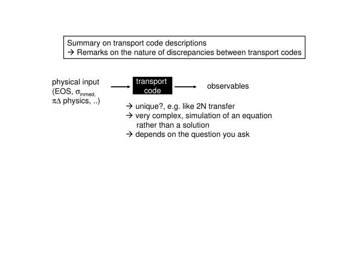
Summary on transport code descriptions Remarks on the nature of discrepancies between transport codes transport code physical input (EOS, σinmed, π∆ physics, ..)

• bservables

unique?, e.g. like 2N transfer very complex, simulation of an equation rather than a solution depends on the question you ask

Transport theory based on a chain of approximations Martin-Schwinger hierachy in many body densities: truncation, introduction of self energies (1-body quantities) Quantum transport theory: Irreversibility, Kadanoff Baym theory semiclassical approximation : Wigner transform, not necc. Phase space probabilities Gradient approximation (sep.of short and long scales) Quasiparticle approximation Spectral function delta function with effective quantities BUU equation

[ ]

) ' f 1 )( f 1 ( f f ) f 1 )( f 1 ( f f ) p p p p ( ) 2 ( ) ( v v d v d v d ) t ; p , r ( f ) r ( U f m p t f

2 ' 1 2 1 2 1 ' 2 ' 1 ' 2 ' 1 2 1 3 12 21 ' 2 ' 1 2 ) p ( ) r (

− − − − − − − + = ∇ ∇ − ∇ + ∂ ∂

∫

δ δ δ δ π π π π Ω Ω Ω Ω σ σ σ σ

• )

t , p , r ( f ) δ δ δ δ +

fluctuations variance of 2b collisions neglct of higher orders 6-dim integro-differential equation, non-linear simulate solutions introduces many technical details

[ ]

) ' f 1 )( f 1 ( f f ) f 1 )( f 1 ( f f ) p p p p ( ) 2 ( ) ( v v d v d v d ) t ; p , r ( f ) r ( U f m p t f

2 ' 1 2 1 2 1 ' 2 ' 1 ' 2 ' 1 2 1 3 12 21 ' 2 ' 1 2 ) p ( ) r (

− − − − − − − + = ∇ ∇ − ∇ + ∂ ∂

∫

δ δ δ δ π π π π Ω Ω Ω Ω σ σ σ σ

• Boltzmann-Vlasov-like (BUU)

solve as exactly as possible:

• test particle method

exact in the limit of NTP∞

• deterministic, no fluctuations

include fluctuations explicitely

• connection between U and σ

by approx of self energy, e.g. Brueckner theory methods of solutions: Molecular dynamic-like (QMD)

• inject classical flcuctuations

and correlations (nucleon wave packet)

• damped (finite Gausians,

averaging width ∆x, parameter + Pauli correlations (AMD)

• relation between U and σ not so clear,

biggest difference: role of fluctuations fragmentation, correlation functions but also affects Pauli blocking and collective excitations

QMD!!!

• Fluctuations: almost a „fight“ between MD and Boltzmann models:

fluc coll

I I dt df + =

now discussed beyond ideological barriers

QMD ZX LI ImQMD

QMD Frankfurt

IQMD

UrQMD LQMD CoMD ImIQMD

SINAP QMD BNU QMD GXNU QMD XY QMD CIAE QMD Sky QMD Tu QMD Z QMD

? ? ? ? ? ? ? ? ? ? ? ? ? ? ? ? AMD

„.. in full bloom…“ – a good sign for the expanding activity, but try to make realtion and changes transparent,

IBUU pBUU GiBUU RBUU RVUU

ImIBUU

SMF SMASH ? BLOB

„…lots of individuals…“

Steps in solving transport simulation

• initialization
• propagation of (test) particles (Vlasov)
• Collision partners and probabilities, elastic (Boltzmann)
• Pauli blocking (Ühling-Uhlenbeck)
• inelastic collisions (new particles), often perturbative, dep. on energy

Code comparison:

• differences of results of codes, e.g. isospin duffusion, pion ratios
• 1. phase: comparison of HIC with controlled input
• differences seen (talk of Betty)
• indications of reasons (initialization, Pauli blocking)
• but difficult to pin point
• general systematic theoretical error (30% (100 MeV), 13% (400 MeV)

how to improve?

• 2. phase: box calculations
• better controlled conditions
• exact limits often available
• resolve differences because of strategies and of errors

from inrinsic differences (like BUU vs. QMD)

Steps in solving transport simulation

• initialization
• propagation of (test) particles (Vlasov)
• Collision partners and probabilities, elastic (Boltzmann)
• Pauli blocking (Ühling-Uhlenbeck)
• inelastic collisions (new particles), often perturbative, dep. on energy

initialization: solvable,

• initialize consistent with density functional used in transport

so that initial nucleus is a good approximation to the ground state

• more important than having identical density distributions

propagation: hamitonian eom, easy but fluctuation dampen critically collective motions momentum dependence, energy conservation

Second formulation of Homework #2: Longer final time and results given each 0.5-1 fm/c

ρk (t) = ʃ dz sin(kz) ρ(z,t) k = n 2π/L

n = 1

Time evolution of Fourier transform ρk

Larger damping and structureless fluctuations In QMD-like Different oscillation frequency in BUU-like

Collision probabilities: Bertsch prescription: particles collide,

• if their distance is below the interaction length and
• if the reach the distance of closest approach in theis time step
• improve: the same nucleons should not colide again in the next time step

lesson: exact results come from kinetic theory, which makes assumtion in complete independence of collisions and equilibrium not so easy to follow in simulations (not always good) mean free path description: assure mf path from kinetic theory assure agreement limits put perhasp oversimplified in collisions (no equilibrium)

Theoretical results for CT0

Pauli blocking: 1 2 1‘ 2‘

• ccupation probablity f(r,p,t)

local

• but realistically averaged over a volume
• often very large, non-localities
• fluctuations!

consequence: evolution to a MB distribution, f(p) >1 prescription: f≤1 how much this affects a transport simulation not clear, very likely in the initial stages, e.g. pre-eq emission

Fluctuations: biggest differences between families of codes and implementation of codes important: yes! indirect: blocking, mf propagation direct: fragments formation

test also fluctuations and fragmentation

how treated: BV-like Boltzmann-Langevin eq. realizations: BOB, SMF, BLOB MD-like: damped classical fluctuations parameter Dx of wave packets light clusters: another problem, tomorrow afternoon.

freeze out: assumption of a completely equilibrated primary fragment is probably too naive there is still collective motion: expansion perhaps a differential freeze-out, surface layer of an expanding source see e.g. Natowitz experiments check with transport models short range correlations: proposed treatments:

• 1. initialize momentum distribution
• but has to active at every moment
• 2. calculate correlation energy in nuclear matter

and use this as a part of the potential energy

• does not generate high energy particles
• 3. three body collisions, to conserve energy
• difficult