STUDY OF INTERPLY SLIP DURING THERMOFORMING OF CONTINOUS FIBER - PDF document

18 TH INTERNATIONAL CONFERENCE ON COMPOSITE MATERIALS STUDY OF INTERPLY SLIP DURING THERMOFORMING OF CONTINOUS FIBER COMPOSITE MATERIALS E. Gazo-Hanna 1 , A. Poitou 1 , P. Casari 1 , L. Juras 2 1 GeM, Ecole Centrale de Nantes, Nantes, France, 2 Cetim de Nantes, Nantes, France Keywords : friction, thermoplastic, forming, interply slip 1 General Introduction Ano ther approach was presented by Akkerman and al. 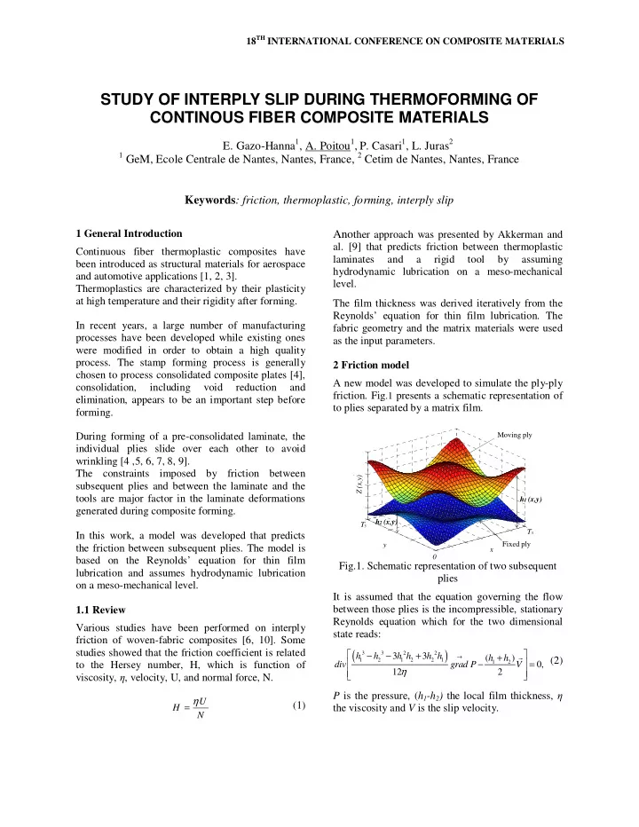[9] that predicts friction between thermoplastic Continuous fiber thermoplastic composites have laminates and a rigid tool by assuming been introduced as structural materials for aerospace hydrodynamic lubrication on a meso-mechanical and automotive applications [1, 2, 3]. level. Thermoplastics are characterized by their plasticity at high temperature and their rigidity after forming. The film thickness was derived iteratively from the Reynolds’ equation for thin film lubrication. The In recent years, a large number of manufacturing fabric geometry and the matrix materials were used processes have been developed while existing ones as the input parameters. were modified in order to obtain a high quality process. The stamp forming process is generally 2 Friction model chosen to process consolidated composite plates [4], A new model was developed to simulate the ply-ply consolidation, including void reduction and friction. Fig .1 presents a schematic representation of elimination, appears to be an important step before to plies separated by a matrix film. forming. Moving ply During forming of a pre-consolidated laminate, the -3 x 10 individual plies slide over each other to avoid 1.6 wrinkling [4 ,5, 6, 7, 8, 9]. 1.4 The constraints imposed by friction between 1.2 Z (x,y) Z(x,y) (cm) subsequent plies and between the laminate and the 1 tools are major factor in the laminate deformations 0.8 h 1 (x,y) 0.6 generated during composite forming. 0.4 h 2 (x,y) T y 6 T x 6 In this work, a model was developed that predicts 4 5 4 3 2 Fixed ply y the friction between subsequent plies. The model is 2 x 1 0 0 0 y (cm) based on the Reynolds’ equation for thin film x (cm) Fig.1. Schematic representation of two subsequent lubrication and assumes hydrodynamic lubrication plies on a meso-mechanical level. It is assumed that the equation governing the flow between those plies is the incompressible, stationary 1.1 Review Reynolds equation which for the two dimensional Various studies have been performed on interply state reads: friction of woven-fabric composites [6, 10]. Some � � studies showed that the friction coefficient is related ( ) 3 3 2 2 � h − h − 3 h h + 3 h h → ( h + h ) (2) � 1 2 1 2 2 1 � 1 2 to the Hersey number, H, which is function of div grad P − V = 0, � � 12 η 2 � � viscosity, � , velocity, U, and normal force, N. P is the pressure, ( h 1 -h 2 ) the local film thickness, � η U (1) = H the viscosity and V is the slip velocity. N

This equation describes the relation between the The friction matrix C f depends on both plies pressure and thickness distribution of a Newtonian geometries, described by h 1 and h 2 , and on the fluid matrix. pressure gradient. The resolution of (equ. 2) is usually made using a 2.1 Model Analyses finite element method. In our case and considering a The previous model shows that the coefficient of periodic profile for h 1 (x,y) and h 2 (x,y) , a pseudo friction is not scalar according to the velocity. spectral method could be used. One boundary After calculating Eigen values � 1 , � 2 and their condition is needed. corresponding Eigen vectors u 1 and u 2 , of matrix C f , we deduced that friction force is only collinear to = (3) P (0,0) 0 velocity when this one is collinear to u 1 or u 2 vectors. �� � �� � It’s important to notice through the writing of the F = λ .( . ) β u Reynolds equation that the pressure depends linearly 1 1 1 �� � �� � (7) on velocity. For this reason, we will try first, and F = λ .( . β u ) 2 2 2 using method described above to solve the Reynolds equation for two different cases where in the first � 1 , � 2 , u 1 and u 2 depend on the film thickness, one, the moving ply slips in the x direction, whereas distribution and regularity. in second case the same ply slips this time in the y direction. The respective solutions will be called y P 1 (x,y) and P 2 (x,y). The linear solution could be written like: � � �� �� � = η + P ( . ( , ) V P x y V P x y . ( , )), (4) u 2 x 1 y 2 F 2 Where V= (V x , V y ) is the velocity vector, x The pressure gradient is calculated: ����� � ����� � ����� � = η + η gradP . . V gradP . V gradP . x 1 y 2 ����� � � � � ����� � �� � � � � � (5) = η ⊗ + ⊗ ⋅ . gradP e gradP e V � � F 1 1 x 2 y � � u 1 = η ⋅ ⋅ M V , ����� � � � � ����� � �� � Fig.2. Schematic representation of friction force Where, M = gradP ⊗ e + gradP ⊗ e when velocity is collinear with u 1 or u 2 1 x 2 y Integrating the shear stress over the sliding surface 3 Numerical results and discussion allows calculating the friction force: The previously presented model (equ.6) was applied → �� to calculate friction parameters between two 3×3 = τ F ( , ) x y dxdy Twill plies as shown in (Fig. 2). x y → + ( h h ) → V �� (6) Geometric equations of both plies are given by: = − 1 2 + η grad P dxdy − 2 h h x y , 1 2 � � � � � � � � 2 π x 2 π y + η ( h h ) �� � � � � * = + ε � � ⋅ h x y ( , ) h 1 cos cos = � − 1 2 M + I dxdy V � ⋅ � � 1 1 1 � � � 2 − � � T � T h h � � � � x y , 1 2 x y (8) � � = C V . � � � � π π f 2 x 2 y � � � � * � � = − ε ⋅ h x y ( , ) h 1 cos cos � � 2 2 2 � � � � This model predicts the friction force F f as a T T � � � � x y function of the friction matrix C f and velocity V .

* , h 2 * , � 1 , � 2 , T x , T y and N, the number of As h 1 collocation points, are the imposed values (Table 1), -3 x 10 P 1 (x,y) , P 2 (x,y), and their respective gradients could 1.6 now be calculated using the pseudo-spectral Fourier 1.4 method. Profiles are shown in (Fig. 4). 1.2 Z(x,y) (cm) 1 Table 1. Example Parameters 0.8 Parameter Value Unit 0.6 * 12.10 -6 h 1 m 0.4 * 6.10 -6 h 2 m 6 � 1 6 0.2 4 5 4 � 2 3 2 0.2 2 1 0 0 T x y (cm) 0.06 m x (cm) T y 0.06 m Fig.3. Inter-ply slip between two 3x3 Twill plies � 100 Pa.s The maximum and the minimum film thicknesses 15 N are equal to: * * = + ε − − ε e h (1 ) h (1 ) max 1 1 2 2 (9) * * e = h (1 − ε ) + h (1 + ε ) min 1 1 2 2 8 8 x 10 5 x 10 x 10 1 1 2 0.5 0.5 1 P2(x,y) (Pa) P1(x,y) (Pa) dP1/dx (N/m) 0 0 0 -0.5 -0.5 -1 -1 -1 -2 8 8 8 6 8 6 8 6 8 6 6 6 4 4 4 4 4 4 2 2 2 2 2 2 0 0 y (cm) 0 0 0 0 y (cm) y (cm) x (cm) x (cm) x (cm) 5 5 5 x 10 x 10 x 10 2 2 2 1 1 1 dP2/dx (N/m) dP1/dy (N/m) dP2/dy (N/m) 0 0 0 -1 -1 -1 -2 -2 -3 -3 -2 8 8 8 6 8 6 8 6 8 6 6 6 4 4 4 4 4 4 2 2 2 2 2 2 0 0 0 y (cm) 0 y (cm) 0 y (cm) 0 x (cm) x (cm) x (cm) Fig.4. Different pressure and gradient of pressure profiles