STK-IN4300 Methods using Derived Input Directions Statistical - - PowerPoint PPT Presentation

SLIDE 1

STK-IN4300 Statistical Learning Methods in Data Science

Riccardo De Bin

debin@math.uio.no

STK-IN4300: lecture 3 1/ 42 STK-IN4300 - Statistical Learning Methods in Data Science

Outline of the lecture

Model Assessment and Selection Cross-Validation Bootstrap Methods Methods using Derived Input Directions Principal Component Regression Partial Least Squares Shrinkage Methods Ridge Regression

STK-IN4300: lecture 3 2/ 42 STK-IN4300 - Statistical Learning Methods in Data Science

Cross-Validation: k-fold cross-validation

The cross-validation aims at estimating the expected test error, Err “ ErLpY, ˆ fpXqqs. ‚ with enough data, we can split them in a training and test set; ‚ since usually it is not the case, we mimic this split by using the limited amount of data we have,

§ split data in K folds F1, . . . , FK, approximatively same size; § use, in turn, K ´ 1 folds to train the model (derive ˆ

f ´kpXq);

§ evaluate the model in the remaining fold,

CV p ˆ f ´kq “ 1 |Fk| ÿ

iPFk

Lpyi, ˆ f ´kpxiqq

§ estimate the expected test error as an average,

CV p ˆ fq “ 1 K

K

ÿ

k“1

1 |Fk| ÿ

iPFk

Lpyi, ˆ f´kpxiqq

|Fk|“ N

K

“ 1 N

N

ÿ

i“1

Lpyi, ˆ f´kpxiqq.

STK-IN4300: lecture 3 3/ 42 STK-IN4300 - Statistical Learning Methods in Data Science

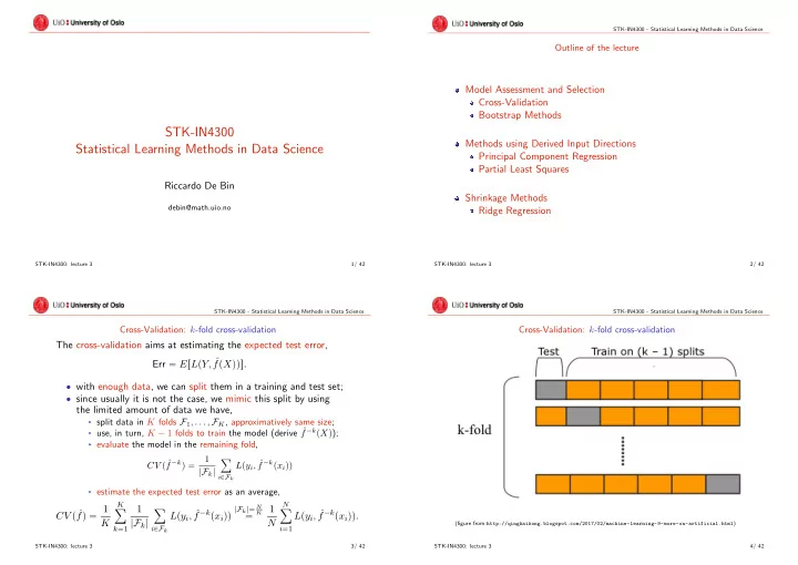
Cross-Validation: k-fold cross-validation

(figure from http://qingkaikong.blogspot.com/2017/02/machine-learning-9-more-on-artificial.html) STK-IN4300: lecture 3 4/ 42

SLIDE 2

STK-IN4300 - Statistical Learning Methods in Data Science

Cross-Validation: choice of K

How to choose K? ‚ there is no a clear solution; ‚ bias-variance trade-off:

§ smaller the K, smaller the variance (but larger bias); § larger the K, smaller the bias (but larger variance); § extreme cases: § K “ 2, half observations for training, half for testing; § K “ N, leave-one-out cross-validation (LOOCV); § LOOCV estimates the expected test error approximatively

unbiased;

§ LOOCV has very large variance (the “training sets” are very

similar to one another);

‚ usual choices are K “ 5 and K “ 10.

STK-IN4300: lecture 3 5/ 42 STK-IN4300 - Statistical Learning Methods in Data Science

Cross-Validation: choice of K

STK-IN4300: lecture 3 6/ 42 STK-IN4300 - Statistical Learning Methods in Data Science

Cross-Validation: further aspects

If we want to select a tuning parameter (e.g., no. of neighbours) ‚ train ˆ f´kpX, αq for each α; ‚ compute CV p ˆ f, αq “ 1

K

řK

k“1 1 |Fk|

ř

iPFk Lpyi, ˆ

f´kpxi, αqq; ‚ obtain ˆ α “ argminαCV p ˆ f, αq. The generalized cross-validation (GCV), GCV p ˆ fq “ 1 N

N

ÿ

i“1

« yi ´ ˆ fpxiq 1 ´ tracepSq{N ff2 ‚ is a convenient approximation of LOOCV for linear fitting under square loss; ‚ has computational advantages.

STK-IN4300: lecture 3 7/ 42 STK-IN4300 - Statistical Learning Methods in Data Science

Cross-Validation: the wrong and the right way to do cross-validation

Consider the following procedure:

• 1. find a subset of good (= most correlated with the outcome)

predictors;

• 2. use the selected predictors to build a classifier;
• 3. use cross-validation to compute the prediction error.

Practical example (see R file): ‚ generated X, an rN “ 50s ˆ rp “ 5000s data matrix; ‚ generate independently yi, i “ 1, . . . , 50, yi P t0, 1u; ‚ the true error test is 0.50; ‚ implementing the procedure above. What does it happen?

STK-IN4300: lecture 3 8/ 42

SLIDE 3

STK-IN4300 - Statistical Learning Methods in Data Science

Cross-Validation: the wrong and the right way to do cross-validation

Why it is not correct? ‚ Training and test sets are NOT independent! ‚ observations on the test sets are used twice. Correct way to proceed: ‚ divide the sample in K folds; ‚ both perform variable selection and build the classifier using

• bservations from K ´ 1 folds;

§ possible choice of the tuning parameter included;

‚ compute the prediction error on the remaining fold.

STK-IN4300: lecture 3 9/ 42 STK-IN4300 - Statistical Learning Methods in Data Science

Bootstrap Methods: bootstrap

IDEA: generate pseudo-samples from the empirical distribution function computed on the original sample; ‚ by sampling with replacement from the original dataset; ‚ mimic new experiments. Suppose Z “ tpx1, y1q loomoon

z1

, . . . , pyN, xNq looomooon

zN

u be the training set: ‚ by sampling with replacement, Z˚

1 “ tpy˚ 1, x˚ 1q

looomooon

z˚

1

, . . . , py˚

N, x˚ Nq

looomooon

z˚

N

u; ‚ . . . . . . . . . . . . . . . . . . . . . ‚ by sampling with replacement, Z˚

B “ tpy˚ 1, x˚ 1q

looomooon

z˚

1

, . . . , py˚

N, x˚ Nq

looomooon

z˚

N

u; ‚ use the B bootstrap samples Z˚

1 , . . . , Z˚ B to estimate any

aspect of the distribution of a map SpZq.

STK-IN4300: lecture 3 10/ 42 STK-IN4300 - Statistical Learning Methods in Data Science

Bootstrap Methods: bootstrap

For example, to estimate the variance of SpZq, x VarrSpZqs “ 1 B ´ 1

B

ÿ

b“1

pSpZ˚

b q ´ ¯

S˚q2 where ¯ S˚ “ 1

B

řB

b“1 SpZ˚ b q.

Note that: ‚ x VarrSpZqs is the Monte Carlo estimate of VarrSpZqs under sampling from the empirical distribution ˆ F.

STK-IN4300: lecture 3 11/ 42 STK-IN4300 - Statistical Learning Methods in Data Science

Bootstrap Methods: bootstrap

STK-IN4300: lecture 3 12/ 42

SLIDE 4

STK-IN4300 - Statistical Learning Methods in Data Science

Bootstrap Methods: estimate prediction error

Very simple: ‚ generate B bootstrap samples Z˚

1 , . . . , Z˚ B;

‚ apply the prediction rule to each bootstrap sample to derive the predictions ˆ f˚

b pxiq, b “ 1, . . . , B;

‚ compute the error for each point, and take the average, x Errboot “ 1 B

B

ÿ

b“1

1 N

N

ÿ

i“1

Lpyi, ˆ f˚

b pxiqq.

Is it correct? NO!!! Again, training and test set are NOT independent!

STK-IN4300: lecture 3 13/ 42 STK-IN4300 - Statistical Learning Methods in Data Science

Bootstrap Methods: example

Consider a classification problem: ‚ two classes with the same number of observations; ‚ predictors and class label independent ñ Err “ 0.5. Using the 1-nearest neighbour: ‚ if yi P Z˚

b Ñ ˆ

Err “ 0; ‚ if yi R Z˚

b Ñ ˆ

Err “ 0.5; Therefore, x Errboot “ 0 ˆ PrrYi P Z˚

b s ` 0.5 ˆ PrrYi R Z˚ b s

looooomooooon

0.368

“ 0.184

STK-IN4300: lecture 3 14/ 42 STK-IN4300 - Statistical Learning Methods in Data Science

Bootstrap Methods: why 0.368

Prrobservation i does not belong to the boostrap sample bs “ 0.368 Since PrrZ˚

brjs ‰ yis “ N ´ 1

N , is true for each position rjs, then PrrYi R Z˚

b s “

ˆN ´ 1 N ˙N

NÑ8

Ý Ý Ý Ý Ñ e´1 « 0.368, Consequently, Prrobservation i is in the boostrap sample bs « 0.632.

STK-IN4300: lecture 3 15/ 42 STK-IN4300 - Statistical Learning Methods in Data Science

Bootstrap Methods: correct estimate prediction error

Note: ‚ each bootstrap sample has N observations; ‚ some of the original observations are included more than once; ‚ some of them (in average, 0.368N) are not included at all;

§ these are not used to compute the predictions; § they can be used as a test set,

x Err

p1q “ 1

N

N

ÿ

i“1

1 |Cr´is| ÿ

bPCr´is

Lpyi, ˆ f˚

b pxiqq

where Cr´is is the set of indeces of the bootstrap samples which do not contain the observation i and |Cr´is| denotes its cardinality.

STK-IN4300: lecture 3 16/ 42

SLIDE 5

STK-IN4300 - Statistical Learning Methods in Data Science

Bootstrap Methods: 0.632 bootstrap

Issue: ‚ the average number of unique observations in the bootstrap sample is 0.632N Ñ not so far from 0.5N of 2-fold CV; ‚ similar bias issues of 2-fold CV; ‚ x Err

p1q slightly overestimates the prediction error.

To solve this, the 0.632 bootstrap estimator has been developed, x Err

p0.632q “ 0.368 Ď

err ` 0.632 x Err

p1q

‚ in practice it works well; ‚ in case of strong overfit, it can break down;

§ consider again the previous classification problem example; § with 1-nearest neighbour, Ď

err “ 0;

§ x

Err

p0.632q “ 0.632 x

Err

p1q “ 0.632 ˆ 0.5 “ 0.316 ‰ 0.5.

STK-IN4300: lecture 3 17/ 42 STK-IN4300 - Statistical Learning Methods in Data Science

Bootstrap Methods: 0.632+ bootstrap

Further improvement, 0.632+ bootstrap: ‚ based on the no-information error rate γ; ‚ γ takes into account the amount of overfitting; ‚ γ is the error rate if predictors and response were independent; ‚ computed by considering all combinations of xi and yi, ˆ γ “ 1 N

N

ÿ

i“1

1 N

N

ÿ

i1“1

Lpyi, ˆ fpxi1qq.

STK-IN4300: lecture 3 18/ 42 STK-IN4300 - Statistical Learning Methods in Data Science

Bootstrap Methods: 0.632+ bootstrap

The quantity ˆ γ is used to estimate the relative overfitting rate, ˆ R “ x Err

p1q ´ Ď

err ˆ γ ´ Ď err , which is then use in the 0.632+ bootstrap estimator, x Err

p0.632`q “ p1 ´ ˆ

wq Ď err ` ˆ w x Err

p1q,

where ˆ w “ 0.632 1 ´ 0.368 ˆ R .

STK-IN4300: lecture 3 19/ 42 STK-IN4300 - Statistical Learning Methods in Data Science

Methods using Derived Input Directions: summary

‚ Principal Components Regression ‚ Partial Least Squares

STK-IN4300: lecture 3 20/ 42

SLIDE 6

STK-IN4300 - Statistical Learning Methods in Data Science

Principal Component Regression: singular value decomposition

Consider the singular value decomposition (SVD) of the N ˆ p (standardized) input matrix X, X “ UDV T where: ‚ U is the N ˆ p orthogonal matrix whose columns span the column space of X; ‚ D is a p ˆ p diagonal matrix, whose diagonal entries d1 ě d2 ě ¨ ¨ ¨ ě dp ě 0 are the singular values of X; ‚ V is the p ˆ p orthogonal matrix whose columns span the row space of X.

STK-IN4300: lecture 3 21/ 42 STK-IN4300 - Statistical Learning Methods in Data Science

Principal Component Regression: principal components

Simple algebra leads to XT X “ V D2V T , the eigen decomposition of XT X (and, up to a constant N, of the sample covariance matrix S “ XT X{N). Using the eigenvectors vj (columns of V ), we can define the principal components of X, zj “ Xvj. ‚ the first principal component z1 has the largest sample variance (among all linear combinations of the columns of X); Varpz1q “ VarpXv1q “ d2

1

N ‚ since d1 ě ¨ ¨ ¨ ě dp ě 0, then Varpz1q ě ¨ ¨ ¨ ě Varpzpq.

STK-IN4300: lecture 3 22/ 42 STK-IN4300 - Statistical Learning Methods in Data Science

Principal Component Regression: principal components

STK-IN4300: lecture 3 23/ 42 STK-IN4300 - Statistical Learning Methods in Data Science

Principal Component Regression: principal components

Principal component regression (PCR): ‚ use M ď p principal components as input; ‚ regress y on z1, . . . , zM; ‚ since the principal components are orthogonal, ˆ ypcrpMq “ ¯ y `

M

ÿ

m“1

ˆ θmzm, where ˆ θm “ xzm, yy{xzm, zmy. Since zm are linear combinations of xj, ˆ βpcrpMq “

M

ÿ

m“1

ˆ θmvm.

STK-IN4300: lecture 3 24/ 42

SLIDE 7

STK-IN4300 - Statistical Learning Methods in Data Science

Principal Component Regression: remarks

Note that: ‚ PCR can be used in high-dimensions, as long as M ă n; ‚ idea: remove the directions with less information; ‚ if M “ N, ˆ βpcrpMq “ ˆ βOLS; ‚ M is a tuning parameter, may be chosen via cross-validation; ‚ shrinkage effect (clearer later); ‚ principal component are scale dependent, it is important to standardize X!

STK-IN4300: lecture 3 25/ 42 STK-IN4300 - Statistical Learning Methods in Data Science

Partial Least Squares: idea

Partial least square (PLS) is based on an idea similar to PCR: ‚ construct a set of linear combinations of X; ‚ PCR only uses X, ignoring y; ‚ in PLS we want to also consider the information on y; ‚ as for PCR, it is important to first standardize X.

STK-IN4300: lecture 3 26/ 42 STK-IN4300 - Statistical Learning Methods in Data Science

Partial Least Squares: algorithm

• 1. standardize each xj, set ˆ

yr0s “ ¯ y and xr0s

j

“ xj;

• 2. For m “ 1, 2, . . . , p,

(a) zm “ řp

j“1 ˆ

ϕmjxrm´1s

j

, with ˆ ϕmj “ xxrm´1s

j

, yy; (b) ˆ θm “ xzm, yy{xzm, zmy; (c) ˆ yrms “ ˆ yrm´1s ` ˆ θzm; (d) orthogonalize each xrm´1s

j

with respect to zm, xrms

j

“ xrm´1s

j

´ ˜ xzm, xrm´1s

j

y xzm, zmy ¸ zm, j “ 1, . . . , p;

• 3. output the sequence of fitted vectors tˆ

yrmsup

1.

STK-IN4300: lecture 3 27/ 42 STK-IN4300 - Statistical Learning Methods in Data Science

Partial Least Squares: step by step

First step: (a) compute the first PLS direction, z1 “ řp

j“1 ˆ

ϕ1jxj,

§ based on the relation between each xj and y, ˆ

ϕ1 “ xxj, yy;

(b) estimate the related regression coefficient, ˆ θ1 “ xz1,yy

xz1,z1y “ Ě z1y Ď z2

1 ;

(c) model after the first iteration: ˆ yr1s “ ¯ y ` ˆ θ1z1; (d) orthogonalize x1, . . . , xp w.r.t. z1, xr2s

j

“ xj ´ ´

xz1,xjy xz1,z1y

¯ z1; We are now ready for the second step . . .

STK-IN4300: lecture 3 28/ 42

SLIDE 8

STK-IN4300 - Statistical Learning Methods in Data Science

Partial Least Squares: step by step

. . . using xr2s

j

instead of xj: (a) compute the second PLS direction, z2 “ řp

j“1 ˆ

ϕ2jxr2s

j ,

§ based on the relation between each xr2s

j

and y, ˆ ϕ2 “ xxr2s

j , yy;

(b) estimate the related regression coefficient, ˆ θ2 “ xz2,yy

xz2,z2y;

(c) model after the second iteration: ˆ yr2s “ ¯ y ` ˆ θ1z1 ` ˆ θ2z2; (d) orthogonalize xr2s

1 , . . . , xr2s p

w.r.t. z2, xr2s

j

“ xr2s

j

´ ˆ

xz2,xr2s

j y

xz2,z2y

˙ z2; and so on, until the M ď p step Ñ M derived inputs.

STK-IN4300: lecture 3 29/ 42 STK-IN4300 - Statistical Learning Methods in Data Science

Partial Least Squares: PLS versus PCR

Differences: PCR the derived input directions are the principal components of X, constructed by looking at the variability of X; PLS the input directions take into consideration both the variability of X and the correlation between X and y. Mathematically: PCR maxαVarpXαq, s.t.

§ ||α|| “ 1 and αT Svℓ “ 0, ℓ “ 1, . . . , M ´ 1;

PLS maxαCor2py, XαqVarpXαq, s.t.

§ ||α|| “ 1 and αT Sϕℓ “ 0, @ℓ ă M.

In practice, the variance tends to dominate Ñ similar results!

STK-IN4300: lecture 3 30/ 42 STK-IN4300 - Statistical Learning Methods in Data Science

Ridge Regression: historical notes

When two predictors are strongly correlated Ñ collinearity; ‚ in the extreme case of linear dependency Ñ super-collinearity; ‚ in the case of super-collinearity, XT X is not invertible (not full rank); Hoerl & Kennard (1970): XT X Ñ XT X ` λIp, where λ ą 0 and Ip “ ¨ ˚ ˚ ˚ ˝ 1 . . . 1 . . . . . . . . . ... . . . . . . 1 ˛ ‹ ‹ ‹ ‚. With λ ą 0, pXT X ` λIpq´1 exists.

STK-IN4300: lecture 3 31/ 42 STK-IN4300 - Statistical Learning Methods in Data Science

Ridge Regression: estimator

Substituting XT X with XT X ` λIp in the LS estimator, ˆ βridgepλq “ pXT X ` λIpq´1XT y. Alternatively, the ridge estimator can be seen as the minimizer of

N

ÿ

i“1

pyi ´ β0 ´

p

ÿ

j“1

βjxijq2, subject to řp

j“1 β2 j ď t.

Which is the same as ˆ βridgepλq “ argminβ # N ÿ

i“1

pyi ´ β0 ´

p

ÿ

j“1

βjxijq2 ` λ

p

ÿ

j“1

β2

j

+ .

STK-IN4300: lecture 3 32/ 42

SLIDE 9

STK-IN4300 - Statistical Learning Methods in Data Science

Ridge Regression: visually

STK-IN4300: lecture 3 33/ 42 STK-IN4300 - Statistical Learning Methods in Data Science

Ridge Regression: visually

STK-IN4300: lecture 3 34/ 42 STK-IN4300 - Statistical Learning Methods in Data Science

Ridge Regression: remarks

Note: ‚ ridge solution is not equivariant under scaling Ñ X must be standardized before applying the minimizer; ‚ the intercept is not involved in the penalization; ‚ Bayesian interpretation:

§ Yi „ Npβ0 ` xT

i β, σ2q;

§ β „ Np0, τ 2q; § λ “ σ2{τ 2; § ˆ

βridgepλq as the posterior mean.

STK-IN4300: lecture 3 35/ 42 STK-IN4300 - Statistical Learning Methods in Data Science

Ridge Regression: bias

Erˆ βridgepλqs “ ErpXT X ` λIpq´1XT ys “ ErpIp ` λpXT Xq´1q´1 pXT Xq´1XT y loooooooomoooooooon

ˆ βLS

s “ pIp ` λpXT Xq´1q´1 loooooooooooomoooooooooooon

wλ

Erˆ βLSs “ wλβ ù ñ Erˆ βridgepλqs ‰ β for λ ą 0. ‚ λ Ñ 0, Erˆ βridgepλqs Ñ β; ‚ λ Ñ 8, Erˆ βridgepλqs Ñ 0 (without intercept); ‚ due to correlation, λa ą λb œ |ˆ βridgepλq| ą |ˆ βridgepλq|.

STK-IN4300: lecture 3 36/ 42

SLIDE 10

STK-IN4300 - Statistical Learning Methods in Data Science

Ridge Regression: variance

Consider the variance of the ridge estimator, Varrˆ βridgepλqs “ Varrwλ ˆ βLSs “ wλVarrˆ βLSswT

λ

“ σ2wλpXT Xq´1wT

λ .

Then,

Varrˆ βLSs ´ Varrˆ βridgepλqs “ σ2 “ pXT Xq´1 ´ wλpXT Xq´1wT

λ

‰ “ σ2wλ “ pIp ` λpXT Xq´1qpXT Xq´1pIp ` λpXT Xq´1qT ´ pXT Xq´1‰ wT

λ

“ σ2wλ “ ppXT Xq´1 ` 2λpXT Xq´2 ` λ2pXT Xq´3q ´ pXT Xq´1‰ wT

λ

“ σ2wλ “ 2λpXT Xq´2 ` λ2pXT Xq´3q ‰ wT

λ ą 0

(since all terms are quadratic and therefore positive) ù ñ Varrˆ βridgepλqs ĺ Varrˆ βLSs

STK-IN4300: lecture 3 37/ 42 STK-IN4300 - Statistical Learning Methods in Data Science

Ridge Regression: degrees of freedom

Note that the ridge solution is a linear combination of y, as the least squares one: ‚ ˆ yLS “ XpXT Xq´1XT loooooooomoooooooon

H

y Ý Ñ d f “ tracepHq “ p; ‚ ˆ yridge “ XpXT X ` λIpq´1XT looooooooooooomooooooooooooon

Hλ

y Ý Ñ d fpλq “ tracepHλq;

§ tracepHλq “ řp

i“1 d2

j

d2

j`λ;

§ dj is the diagonal element of D in the SVD of X; § λ Ñ 0, d

fpλq Ñ p;

§ λ Ñ 8, d

fpλq Ñ 0.

STK-IN4300: lecture 3 38/ 42 STK-IN4300 - Statistical Learning Methods in Data Science

Ridge Regression: more about shrinkage

Recall the SVD decomposition X “ UDV T , and the properties U T U “ Ip “ V T V. ˆ βLS “ pXT Xq´1XT y “ pV DU T UDV T q´1V DU T y “ pV D2V T q´1V DU T y “ V D´2V T V DU T y “ V D´2DU T y ˆ yLS “ X ˆ βLS “ UDV T V D´2DUT y “ UDD´2DU T y “ UU T y

STK-IN4300: lecture 3 39/ 42 STK-IN4300 - Statistical Learning Methods in Data Science

Ridge Regression: more about shrinkage

ˆ βridge “ pXT X ` λIpq´1XT y “ pV DU T UDV T ` λIpq´1V DU T y “ pV D2V T ` λV V T q´1V DU T y “ V pD2 ` λIpq´1V T V DU T y “ V pD2 ` λIpq´1U T y ˆ yridge “ X ˆ βridge “UDV T V pD2 ` λIpq´1U T y “UV T V D2pD2 ` λIpq´1U T y “U D2pD2 ` λIpq´1 looooooooomooooooooon U T y

p

ÿ

j“1

d2

j

d2

j ` λ

So: ‚ small singular values dj correspond to directions of the column space of X with low variance; ‚ ridge regression penalizes the most these directions.

STK-IN4300: lecture 3 40/ 42

SLIDE 11

STK-IN4300 - Statistical Learning Methods in Data Science

Ridge Regression: more about shrinkage

(picture from https://onlinecourses.science.psu.edu/stat857/node/155/)

STK-IN4300: lecture 3 41/ 42 STK-IN4300 - Statistical Learning Methods in Data Science

References I

Hoerl, A. E. & Kennard, R. W. (1970). Ridge regression: Biased estimation for nonorthogonal problems. Technometrics 12, 55–67.

STK-IN4300: lecture 3 42/ 42