STK-IN4300 Piecewise polynomials and splines Smoothing splines - PowerPoint PPT Presentation

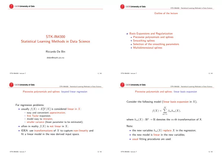
STK-IN4300 - Statistical Learning Methods in Data Science Outline of the lecture Basis Expansions and Regularization STK-IN4300 Piecewise polynomials and splines Smoothing splines Statistical Learning Methods in Data Science Selection of the smoothing parameters Multidimensional splines Riccardo De Bin debin@math.uio.no STK-IN4300: lecture 7 1/ 43 STK-IN4300: lecture 7 2/ 43 STK-IN4300 - Statistical Learning Methods in Data Science STK-IN4300 - Statistical Learning Methods in Data Science Piecewise polynomials and splines: beyond linear regression Piecewise polynomials and splines: linear basis expansion Consider the following model (linear basis expansion in X ), For regression problems: M ‚ usually f p X q “ E r Y | X s is considered linear in X : ÿ f p X q “ β m h m p X q , § easy and convenient approximation; m “ 1 § first Taylor expansion; where h m p X q : R p Ñ R denotes the m -th transformation of X. § model easy to interpret; § smaller variance (fewer parameter to be estimated); ‚ often in reality f p X q is not linear in X ; Note: ‚ the new variables h m p X q replace X in the regression; ‚ IDEA: use transformations of X to capture non-linearity and fit a linear model in the new derived input space. ‚ the new model is linear in the new variables; ‚ usual fitting procedures are used. STK-IN4300: lecture 7 3/ 43 STK-IN4300: lecture 7 4/ 43

STK-IN4300 - Statistical Learning Methods in Data Science STK-IN4300 - Statistical Learning Methods in Data Science Piecewise polynomials and splines: choices of h m p X q Piecewise polynomials and splines: introduction Remarks: ‚ particular functional forms (e.g., logarithm) are useful in Typical choices of h m p X q : specific situations; ‚ polynomial forms are more flexible but limited by their global ‚ h m p X q “ X m : original linear model; nature; ‚ h m p X q “ X 2 j or h m p X q “ X j X k : polynomial terms, § augmented space to achieve higher-order Taylor expansions; § the number of variables grows exponentially ( O p p d q , where d is ‚ piecewise-polynomials and splines allow for local polynomials; the order of the polynomial, p the number of variables); ‚ the class of functions is limited, a ‚ h m p X q “ log p X j q , X j , . . . : non-linear transformations; p ÿ f p X q “ f j p X j q ‚ h m p X q “ 1 p L m ď X k ă U m q : indicator for a region of X k , j “ 1 § breaks the range of X k into M k non-overlapping regions; § piecewise constant contribution of X k . p M ÿ ÿ “ β jm h jm p X j q , j “ 1 m “ 1 by the number of basis M j used for each component f j . STK-IN4300: lecture 7 5/ 43 STK-IN4300: lecture 7 6/ 43 STK-IN4300 - Statistical Learning Methods in Data Science STK-IN4300 - Statistical Learning Methods in Data Science Piecewise polynomials and splines: piecewise constant Piecewise polynomials and splines: piecewise linear The piecewise constant A piecewise linear fit: function: ‚ a linear fit instead of a ‚ simplest solution; constant fit in each region; ‚ three basis functions: ‚ three additional basis § h 1 p X q “ 1 p X ă ξ 1 q functions: § h 2 p X q “ 1 p ξ 1 ď X ă ξ 2 q § h 4 p X q “ h 1 p X q X § h 3 p X q “ 1 p ξ 2 ď X q § h 5 p X q “ h 2 p X q X ‚ disjoint regions; § h 6 p X q “ h 3 p X q X ‚ f p X q “ ř 3 m “ 1 β m h m p X q ; ‚ ˆ β 1 , ˆ β 2 , ˆ β 3 are the intercepts; ‚ ˆ β m “ ¯ Y m , the mean of Y in ‚ ˆ β 4 , ˆ β 5 , ˆ β 6 are the slopes; the region m . STK-IN4300: lecture 7 7/ 43 STK-IN4300: lecture 7 8/ 43

STK-IN4300 - Statistical Learning Methods in Data Science STK-IN4300 - Statistical Learning Methods in Data Science Piecewise polynomials and splines: piecewise linear Piecewise polynomials and splines: piecewise linear The constraint can be directly A continuous piecewise linear fit: incorporated into the basis ‚ force continuity at knots; functions, ‚ generally preferred to the ‚ h 1 p X q “ 1 non-continuous version; ‚ h 2 p X q “ X ‚ add constraints, § ˆ β 1 ` ξ 1 ˆ β 4 “ ˆ β 2 ` ξ 1 ˆ ‚ h 3 p X q “ p X ´ ξ 1 q ` β 5 ; § ˆ β 2 ` ξ 2 ˆ β 5 “ ˆ β 3 ` ξ 2 ˆ β 6 ; ‚ h 4 p X q “ p X ´ ξ 2 q ` ‚ 2 restrictions Ñ 4 free where p¨q ` denotes the positive parameters; part. STK-IN4300: lecture 7 9/ 43 STK-IN4300: lecture 7 10/ 43 STK-IN4300 - Statistical Learning Methods in Data Science STK-IN4300 - Statistical Learning Methods in Data Science Piecewise polynomials and splines: piecewise cubic polynomials Piecewise polynomials and splines: piecewise cubic polynomials Further “improvements”: Also in this case: ‚ smoother functions; ‚ we can force the function to ‚ increase the order of the be continuous at the nodes; polynomials; ‚ by adding constrains; ‚ e.g., a cubic polynomial in each disjoint region; Ó Ó continuous piecewise cubic polynomials. discontinuous piecewise cubic polynomials. STK-IN4300: lecture 7 11/ 43 STK-IN4300: lecture 7 12/ 43

STK-IN4300 - Statistical Learning Methods in Data Science STK-IN4300 - Statistical Learning Methods in Data Science Piecewise polynomials and splines: piecewise cubic polynomials Piecewise polynomials and splines: piecewise cubic polynomials Finally, ‚ further increase the order of Since we have third order continuity; polynomials: ‚ constrain f 2 p ξ ´ k q “ f 2 p ξ ` k q ‚ we can increase the order of Ó continuity at knots; ‚ not only f p ξ ´ k q “ f p ξ ` cubic splines . k q ; ‚ additionally, f 1 p ξ ´ k q “ f 1 p ξ ` k q . Ó Basis for cubic splines with two first derivative continuous knots ξ 1 and ξ 2 : piecewise cubic polynomials. h 3 p X q “ X 2 , h 5 p X q “ p X ´ ξ 1 q 3 h 1 p X q “ 1 , ` h 4 p X q “ X 3 , h 6 p X q “ p X ´ ξ 2 q 3 h 2 p X q “ X , ` STK-IN4300: lecture 7 13/ 43 STK-IN4300: lecture 7 14/ 43 STK-IN4300 - Statistical Learning Methods in Data Science STK-IN4300 - Statistical Learning Methods in Data Science Piecewise polynomials and splines: general order-M splines Piecewise polynomials and splines: specifications For this kind of splines (a.k.a. regression splines), one needs to: In general, an order-M spline with knots ξ j , j “ 1 , . . . , K : ‚ is a piecewise-polynomial of degree M ´ 1 ; ‚ specify the order of the spline; ‚ has continuous derivatives up to order M ´ 2 ; ‚ select the number of the knots; ‚ choose their placement. ‚ the general form of the basis is: Often: h j p X q “ X j ´ 1 , j “ 1 , . . . , M ; ‚ use cubic splines ( M “ 4 ); h M ` ℓ p X q “ p X ´ ξ ℓ q M ´ 1 , ℓ “ 1 , . . . , K ; ` ‚ use the degrees of freedom to choose the number of knots; ‚ e.g., for cubic splines, ‚ e.g., cubic spline Ñ M “ 4 ; § 4 degrees of freedom for the first cubic polynomial; ‚ cubic splines are the lowest-order spline for which the § 1 degree of freedom for each knot ( 4 ´ 1 ´ 1 ´ 1 ); discontinuity at the knots cannot be seen by a human eye § number of basis = number of knots + 4; ó ‚ use the x i to place the knots; § e.g., with 4 knots, 20 th , 40 th , 60 th , 80 th percentiles of x . no reason to use higher-order splines STK-IN4300: lecture 7 15/ 43 STK-IN4300: lecture 7 16/ 43

STK-IN4300 - Statistical Learning Methods in Data Science STK-IN4300 - Statistical Learning Methods in Data Science Piecewise polynomials and splines: natural cubic splines Piecewise polynomials and splines: natural cubic splines At the boundaries: ‚ same issues seen for kernel density; ‚ high variance. Solution: ‚ force the function to be linear beyond the boundary knots; ‚ by adding additional constraints; ‚ it frees up 4 (2 for each boundary) degrees of freedom. Basis (derived from those of the cubic splines): N 1 p X q “ 1 N 2 p X q “ X N k ` 2 p X q “ d k p X q ´ d K ` 1 where d k “ p X ´ ξ k q 3 ` ´ p X ´ ξ K q 3 ` . ξ K ´ ξ k STK-IN4300: lecture 7 17/ 43 STK-IN4300: lecture 7 18/ 43 STK-IN4300 - Statistical Learning Methods in Data Science STK-IN4300 - Statistical Learning Methods in Data Science Piecewise polynomials and splines: example Piecewise polynomials and splines: example STK-IN4300: lecture 7 19/ 43 STK-IN4300: lecture 7 20/ 43